Neural Radiance Fields: A Comprehensive Review 📚🔍✨

This blog offers a comprehensive exploration of Neural Radiance Fields (NeRFs), a method for photorealistic 3D scene reconstruction from sparse 2D images. It covers foundational concepts, training techniques, and notable advancements and well-known variants in the NeRF family.

Table of Contents

1. Introduction to NeRFs
   1.1 Scene Representation
   1.2 Volume Rendering
   1.3 Architectures
   1.4 Why Neural Fields?

2. Training and Optimization
   2.1 Ray Sampling
   2.2 Volume Rendering
   2.3 Loss Calculation and Optimization
   2.4 Optimization
   2.5 Regularization Techniques
3. Quality Assessment Metrics
4. NeRF Zoo 4.1 Mip-NeRF
   4.2 Mip-NeRF 360 4.3 NeRF-W 4.4 DS-NeRF 4.5 DDP-NeRF 4.6 Plenoxels

1. Introduction to NeRFs

Neural Radiance Fields (NeRF) was introduced by Mildenhall et al. in 2020 as a transformative method for synthesizing novel views of a 3D scene using only a sparse collection of 2D input images.

By learning a continuous volumetric representation, NeRF enables the generation of photorealistic images from arbitrary viewpoints.

This capability has positioned NeRF as a pivotal technique in computer vision and graphics, with applications spanning virtual reality, augmented reality, and visual effects.

1.1 Scene Representation

NeRF represents a 3D scene as a continuous 5D function $F_\Theta$ that maps spatial coordinates ($x$) and viewing directions ($\theta, \phi$) to color ($c$) and density ($\sigma$):

Inputs:

• 3D Spatial Coordinates ($x = (x, y, z) \in \mathbb{R}^3$): Define the position of a point in the scene.
• 2D Viewing Directions ($d = (\theta, \phi) \in \mathbb{R}^2$): Specify how the point appears from a particular viewpoint, often converted into 3D Cartesian unit vectors ($d = (d_x, d_y, d_z)$) for simplicity.

Outputs:

• Color ($c = (r, g, b) \in \mathbb{R}^3$): The RGB value representing the appearance of the point.
• Density ($\sigma \in \mathbb{R}$): Indicates the opacity or solidity of the point.

Through this formulation, NeRF learns both the geometry and appearance of a 3D scene. This enables the model to generate a sequence of novel views by querying the learned function at arbitrary spatial coordinates and viewing directions.

1.2 Volume Rendering

To synthesize 2D images from the learned 3D representation, NeRF employs volume rendering, a process that integrates color and density along camera rays cast into the scene. A ray is parameterized as:

Where:

• $r_0$: The origin of the camera.
• $t$: The depth along the ray.
• $d$: The direction of the ray.

The color of a pixel is approximated by summing the contributions of sampled points along the ray:

Where:

• $C_i$: The color at the $i$-th sampled point.
• $\sigma_i$: The density at the $i$-th sampled point, representing its contribution to the ray’s opacity.
• $T_i$: The transmittance, describing the fraction of light that reaches the $i$-th point without being absorbed by prior points along the ray.

This formulation allows NeRF to render realistic images by simulating the interaction of light with the scene, capturing complex lighting effects, shadows, and reflections.

1.3 Positional Encoding

To capture fine details and high-frequency variations in scenes, NeRF uses positional encoding to transform the spatial coordinates $x$ and viewing directions $d$ into higher-dimensional representations. We can use sinusoidal positional encoding to encode the input features:

Where:

• $L$: Determines the number of frequencies used for encoding.

This encoding enables the model to learn high-frequency scene details, such as sharp edges and fine lighting patterns.

1.4 Architecture

NeRF’s architecture revolves around a Multilayer Perceptron (MLP), a fully connected neural network designed to map input features to outputs with the following structure:

• Input Encoding: Spatial coordinates $x$ and viewing directions $d$ are preprocessed using positional encoding.

• Network Structure: 8 hidden layers: Each with 256 neurons and ReLU activation. A skip connection is added after the 5th layer to improve information flow and address the vanishing gradient problem.

• Density Head: predicts the Density ($\sigma$) and a 256-dimensional feature vector for the color prediction.

• Color Head: Combines the feature vector with the positional encoding of the viewing direction ($d$) to predict the final color ($c$).

This architectural design balances computational efficiency with representational power, enabling NeRF to model complex geometries, lighting effects, and subtle scene details.

1.5 Why Neural Fields?

Neural fields models have several key advantages over traditional 3D representation methods:

• Compactness: Encodes an entire scene into a compact, continuous function, significantly reducing memory requirements compared to voxel grids, meshes, or point clouds.
• Regularization: Neural fields inherently produce smooth and coherent outputs by interpolating sparse input data, effectively reducing noise and overfitting.
• Domain Agnostics: Works directly with sparse 2D images, allowing generalization across diverse scenes without the need for explicit 3D supervision or dense datasets.

These advantages make neural fields, including NeRF, highly impactful in rendering, 3D scene reconstruction, and numerous applications in computer vision and graphics.

2. Training and Optimization

Training Neural Radiance Fields (NeRFs) involves learning to represent a scene by minimizing the difference between the rendered outputs and ground truth images. This is achieved using a differentiable volume rendering pipeline. NeRF optimizes a neural network to predict both the density ($\sigma$) and color ($\mathbf{c}$) at sampled 3D points, which are then aggregated to render realistic 2D images.

2.1 Ray Sampling

To model the scene, NeRF operates on rays emitted from the camera. Each pixel in the input image corresponds to a single ray, parameterized as:

Where:

• $\mathbf{o}$: Camera origin.
• $\mathbf{d}$: Direction of the ray.
• $t$: Depth parameter, with $t_{\text{n}} \leq t \leq t_{\text{f}}$ for near and far bounds.

The ray is divided into $N$ uniformly spaced intervals, $t$, producing sampled points along the ray:

Thus, for each $ t_k \in t $, we compute its corresponding 3D position along the ray $ x = r(t_k) $, and transform each position into a higher-dimensional representation using positional encoding $\gamma(x)$, $ \gamma(r(t_k)) $.

The network then predicts the density $\sigma_i$ and color $\mathbf{c}_i$ at each sampled point as:

During training, the sampling is stochastic, but during inference, the sampling is evenly spaced between $ t_{\text{n}} $ and $ t_{\text{f}} $.

To improve efficiency, NeRF employs a coarse-to-fine sampling strategy:

• Coarse Network: Samples points uniformly to estimate the rough density distribution along the ray.
• Fine Network: Focuses additional samples in regions with high density, improving accuracy in critical areas.

Hierarchical sampling enables NeRF to allocate computational resources efficiently, avoiding unnecessary evaluations in empty spaces.

2.2 Volume Rendering

Volume rendering integrates the contributions of sampled points along a ray to compute the final color of a pixel. The pixel color is defined as:

Where:

• $T_i = \prod_{j=1}^{i-1} (1 - \alpha_j)$: Transmittance, representing how much light reaches the $i$-th point without being absorbed.
• $\alpha_i = 1 - \exp(-\sigma_i \cdot \Delta t)$: Opacity derived from density $\sigma_i$ and spacing $\Delta t$ between samples.
• $\mathbf{c}_i$: Predicted color at the $i$-th point.

We approximate the volume rendering integral using numerical quadrature as:

with

2.3 Loss Calculation and Optimization

The training objective of NeRF is to minimize the rendering loss, which measures the difference between the rendered image and the ground truth image. The loss is defined as:

We minimize the sum of squared differences between all pixel values in the predicted image and the ground truth image using the gradient descent algorithm. NeRF uses two separate networks for coarse $\Theta^{c}$ and fine $\Theta^{f}$ sampling, and the loss function is defined as:

Where:

• $C^{*}(r)$: Ground truth color.
• $C(r, \Theta, t^{c})$: Color predicted by the coarse MLP.
• $C(r, \Theta, \text{sort}(t^{c} \cup t^{f}))$: Color predicted by the fine MLP.
• $\lambda$: Hyperparameter to balance the contributions of the coarse and fine predictions.
• $\mathcal{R}$: Set of rays.

We can extend the loss function with additional terms to improve training:

• Sparsity Regularization:
  Penalizes unnecessary density in empty regions, reducing artifacts: \(\mathcal{L}_{\text{sparsity}} = \lambda \cdot \sum_{i} \exp(-\sigma_i)\)
• Depth Supervision (if available):
  Incorporates depth information to refine density predictions: \(\mathcal{L}_{\text{depth}} = \frac{1}{|\mathcal{R}|} \sum_{r \in \mathcal{R}} \| D(r) - D_{\text{true}}(r) \|^2\)

2.4 Optimization

NeRF’s parameters ($\Theta$) are optimized using gradient-based learning. The optimization process involves:

1. Gradient Descent:
   The network updates its weights iteratively using: \(\Theta \leftarrow \Theta - \eta \cdot \nabla_\Theta \mathcal{L}\) Where:
   • $\eta$: Learning rate.
   • $\nabla_\Theta \mathcal{L}$: Gradient of the loss function with respect to the parameters.
2. Batchifying Rays:
   Rays are processed in batches where each batch is sampled randomly to ensure the network generalizes well across the scene.

2.5 Regularization Techniques

To enhance generalization and avoid overfitting, NeRF employs several regularization methods:

1. Sparsity Constraints:
   Encourages the network to predict zero density in empty regions, reducing noise and artifacts as: \(\mathcal{L}_{\text{sparsity}} = \lambda \cdot \sum_{i} \exp(-\sigma_i)\)

2. Smoothness Regularization:
   Ensures consistent density predictions across nearby sampled points.

3. Depth Supervision:
   If depth data is available, supervising the network with known depth values ensures more accurate density estimation.

Before we delve into the NeRFs variants, let’s explore some quality assessment metrics for evaluating and benchmarking NeRF models.

Quality Assessment Metrics

To evaluate the realism, accuracy, and efficiency of Neural Radiance Fields (NeRFs), several metrics are commonly used to assess and compare different models. These include:

1. PSNR (Peak Signal-to-Noise Ratio):
   Measures the fidelity of the synthesized images compared to ground-truth images, where $ PSNR(I) $ can be calculated as:

Where:

• $ I $: The synthesized image.
• $ \text{Max} $: The Maximum pixel value (e.g., 255 for 8-bit images).
• $ \text{MSE}(I) $: The Mean Squared Error between the synthesized image and the ground truth image, calculated as:
  \(\text{MSE}(I) = \frac{1}{N} \sum_{i=1}^{N} (I_i - I_{\text{GT}_i})^2\)
• $ N $: The total number of pixels in the image.
• $ I_i $: The pixel value in the synthesized image.

• $ I_{\text{GT}_i} $: The corresponding pixel value in the ground truth image.

  A higher $ PSNR $ value indicates better image quality, with less deviation from the ground truth image.

1. SSIM (Structural Similarity Index Metric):
   Evaluates the structural similarity between the synthesized and ground truth images, incorporating luminance, contrast, and structure. The SSIM index can be calculated as:
   \(\text{SSIM}(I, I_{\text{GT}}) = \frac{(2\mu_{I} \mu_{I_{\text{GT}}} + C_1)(2\sigma_{I I_{\text{GT}}} + C_2)}{(\mu_{I}^2 + \mu_{I_{\text{GT}}}^2 + C_1)(\sigma_{I}^2 + \sigma_{I_{\text{GT}}}^2 + C_2)}\)
   Where:
   • $ \mu_{I} $: The mean of the synthesized image.
   • $ \mu_{I_{\text{GT}}} $: The mean of the ground truth image.
   • $ \sigma_{I}^2 $: The variance of the synthesized image.
   • $ \sigma_{I_{\text{GT}}}^2 $: The variance of the ground truth image.
   • $ \sigma_{I I_{\text{GT}}} $: The covariance of the synthesized and ground truth images.
   • $ C_1 $ and $ C_2 $: Constants to stabilize the division with weak denominator.

   \(C_1 = (K_1 L)^2, \quad C_2 = (K_2 L)^2\)
   Where:

   • $ L $: The dynamic range of the pixel values (e.g., 255 for 8-bit images).
   • $ K_1 = 0.01 $ and $ K_2 = 0.03 $ by default.

   The $ \text{SSIM} $ index ranges from -1 to 1, with 1 indicating perfect similarity between the images.

2. LPIPS (Learned Perceptual Image Patch Similarity):

   LPIPS is a perceptual similarity metric that evaluates the visual similarity between images based on deep features extracted from neural networks. It captures both low-level and high-level visual information to compute a perceptual distance between images.

   The LPIPS score is computed as a weighted sum of perceptual distances across different feature map layers. The formula can be expressed as:
   \(\text{LPIPS}(I, I_{\text{GT}}) = \sum_{l=1}^L w_l \cdot \frac{1}{H_l \cdot W_l} \sum_{h=1}^{H_l} \sum_{w=1}^{W_l} \|\phi_l(I)_{h,w} - \phi_l(I_{\text{GT}})_{h,w}\|_2^2\)
   Where:

• $ L $: The total number of feature map layers used from the network.
• $ w_l $: The weight assigned to the perceptual distance at layer $ l $.
• $ H_l $, $ W_l $: The height and width of the feature map at layer $ l $.
• $ \phi_l(I)_{h,w} $: The feature activation of the synthesized image $ I $ at spatial location $ (h, w) $ in layer $ l $.

• $\phi_l(I_{\text{GT}}){h,w}$ : The corresponding feature activation of the ground-truth image $ I{\text{GT}} $ at the same location.

  LPIPS computes the perceptual difference in feature activations spatially, normalizing over the feature map dimensions to ensure consistency across layers of varying resolutions. A lower $ \text{LPIPS} $ score indicates greater perceptual similarity between the synthesized and ground-truth images.

We will also monitor the training time and the inference time to comprehensively evaluate their performance.

4. NeRF Zoo

We are now ready to explore the variants of Neural Radiance Fields (NeRFs) :).

4.1 Mip-NeRF

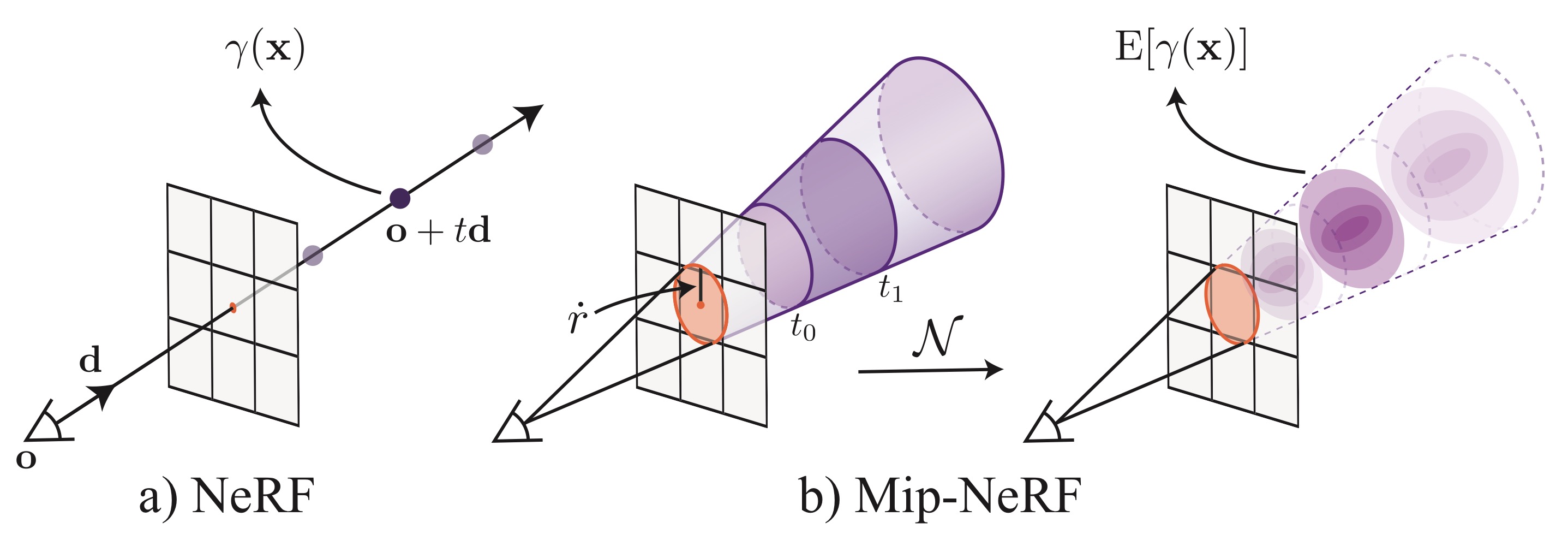
Mip-NeRF uses cone tracing instead of ray tracing in the vanilla NeRF, inspired by mipmapping in computer graphics. NeRF’s point sampling makes it vulnerable to aliasing and sampling blur. Mip-NeRF addresses this issue by casting a cone from each pixel, dividing the cone into a series of canonical frustums, and replacing the positional encoding (PE) with Integrated Positional Encoding (IPE), which represents the volume of the frustum. This allows the model to reason about the size and shape of each canonical frustum instead of its centroid.

In Mip-NeRF, a sorted vector of distances $t$ is defined, and the ray is split into a set of intervals $T_i = [t_i, t_{i+1})$. For each interval $i$, the mean and variance $(\mu, \Sigma) = r(T_i)$ of the canonical frustum corresponding to the interval are computed, where $r(T_i)$ represents the integration process across the frustum. These statistics are then featurized using Integrated Positional Encoding (IPE).

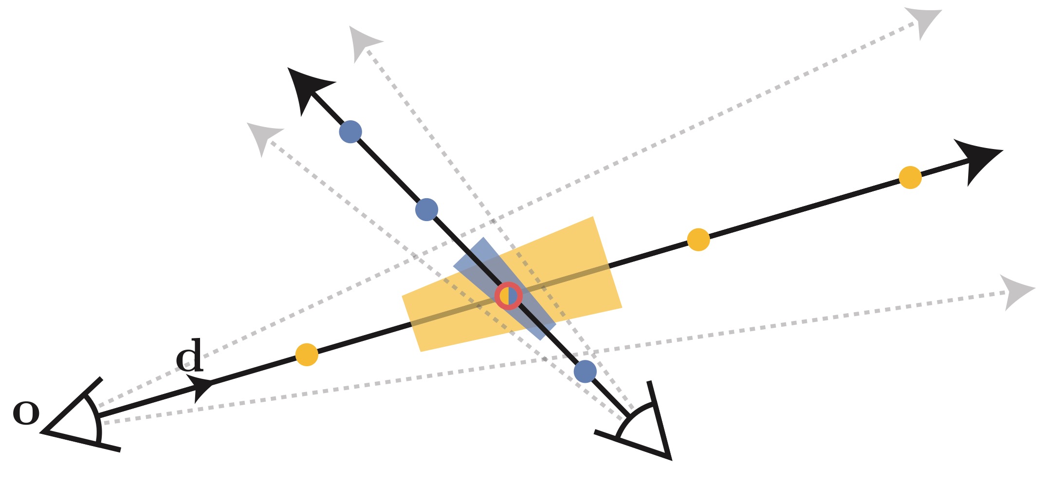
The IPE feature maps the mean and the diagonal of the covariance matrix into higher-dimensional space using sinusoidal functions. The formula for the encoding is:

where $\mu_{\gamma}$ and $\Sigma_{\gamma}$ are the mean and variance lifted into the positional encoding space. This approach captures both the location (mean) and uncertainty (variance) of the interval, enabling multiscale representations by design and reducing aliasing.

The rays are rendred using the distances $t^{c}$ between the intervals $[t_{n}, t_{f}]$, $t^{c} \sim Dist{[t_n, t_f]} $, After the coarse MLP generates the vector of coarse $w^{c}$, fine distances $t^{f}$ are sampled from the histogram defined by $t^{c}$ and the $w^{c}$, using inverse transform sampling $t^{f} \sim Hist(t^{c}, w^{c})$.

Mip-NeRF uses a single MLP, queried repeatedly in a hierarchical sampling approach. This replaces the coarse and fine MLPs of vanilla NeRF, reducing the model size by 50%. This design results in more efficient sampling, improved rendering accuracy, and faster training and inference.

The optimization process balances contributions from coarse and fine predictions with the following reconstruction loss function:

where $\mathcal{R}$ is the set of rays, $C^{*}(r)$ is the ground truth color, $C(r, \boldsymbol{\Theta}, t^{c})$ is the color predicted by the coarse MLP, and $C(r, \boldsymbol{\Theta}, t^{f})$ is the color predicted by the fine MLP. The hyperparameter $\lambda$ (set to $0.1$) ensures proper balancing between the two terms.

By introducing cone tracing, Integrated Positional Encoding, and hierarchical sampling, Mip-NeRF achieves significant improvements in rendering quality and efficiency over vanilla NeRF. It was implemented using JAX, leveraging the same framework as JAXNeRF.

4.2. Mip-NeRF 360

Mip-NeRF 360 is an extension of Mip-NeRF designed to address the challenges of unbounded scenes. It incorporates a nonlinear scene parametrization, online distillation, and a novel distortion-based regularizer to improve performance in such environments. It is specifically designed for scenarios where the camera rotates 360° around a point.

Both NeRF and Mip-NeRF struggle in unbounded scenes, where the camera may face any direction and the scene content may extend to an infinite distance.

• Parametrization

Unbounded scenes can occupy an arbitrarily large region of Euclidean space, requiring a different parametrization than the vanilla NeRF. Thus, a smooth parametrization of volumes rather than points was proposed. To achieve this, let us define $f(x)$ as a mapping function from $\mathbb{R}^3$ to $\mathbb{R}^3$. We can approximate the mapping function linearly at a point $\mu$ as:

where $J_f(\mu)$ is the Jacobian of $f$ at $\mu$. The mapping can be applied to both the mean $\mu$ and the covariance $\Sigma$ as follows:

We choose $f$ as a contraction mapping. If $|x|$ is less than 1, the function is defined as follows:

This design distributes the points proportionally to disparity rather than distance. However, this uniformly spaced design is not suitable for unbounded scenes in all directions. To address this, we define a mapping between the Euclidean space ray distance $t$ and a “normalized” ray distance $s$ as:

where $g(\cdot)$ is some invertible scalar function. For instance, let $g(x) = \frac{1}{x}$, which yields a normalized ray distance $t \in [t_n, t_f]$ mapped to $s \in [0, 1]$ in the form of “inverse depth spacing.”

• Efficiency

Large and detailed scenes require more network capacity and more samples along the ray to accurately model surfaces, resulting in slower training and inference times.

Instead of training two MLPs separately, a “Proposal MLP” $\Theta_{\text{prop}}$ and a “NeRF MLP” $\Theta_{\text{nerf}}$ are trained together. The “Proposal MLP” is used to predict the volumetric density, and those densities $\hat{w}$ are used to sample $s$-intervals. The “NeRF MLP” uses these $s$-intervals to render the final image.

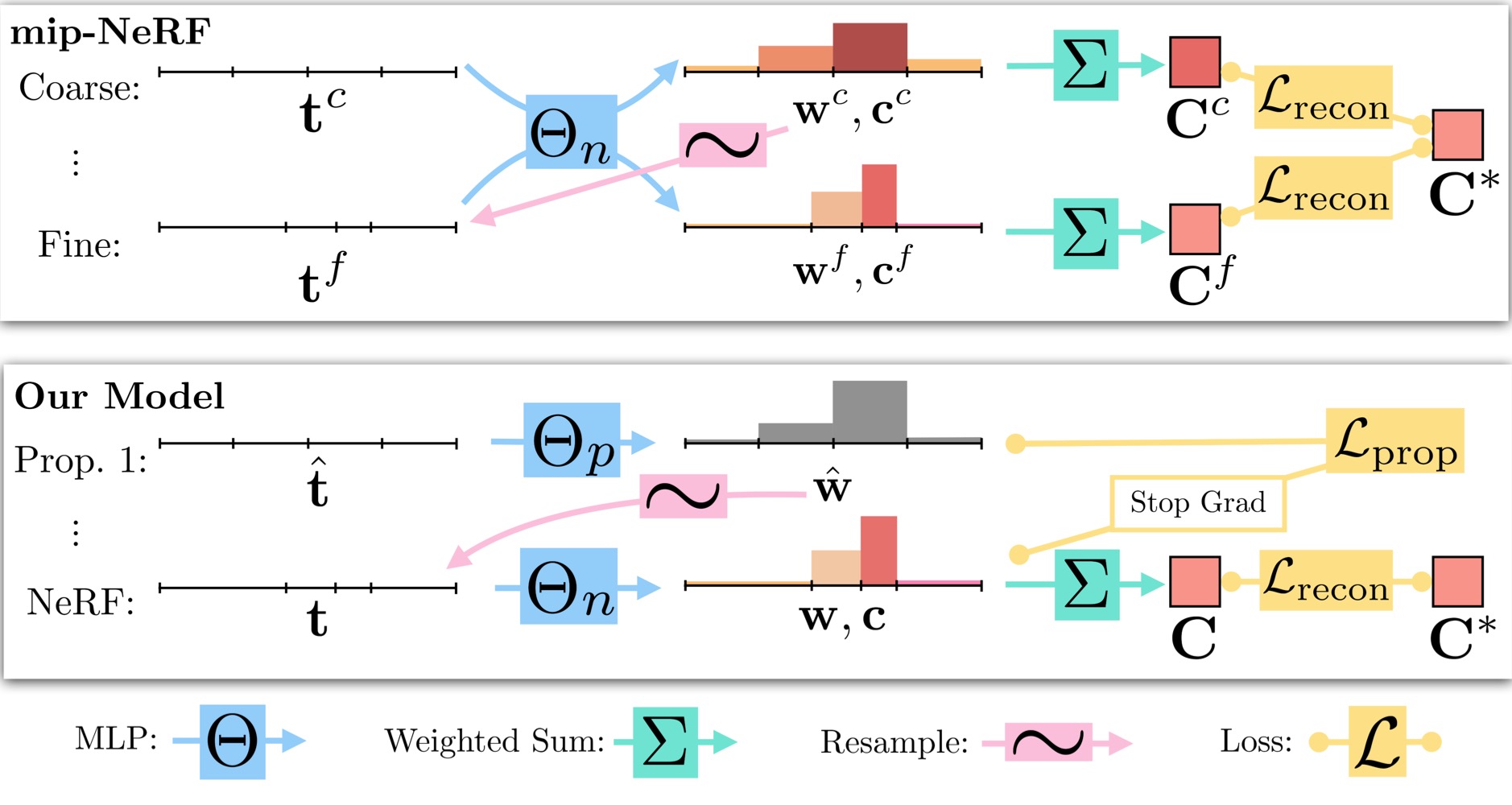
This approach can be seen as a form of online distillation, where both MLPs are initialized randomly and trained jointly. While the “Proposal MLP” is a small model, it does not affect accuracy significantly.

The “Proposal MLP” is sampled and evaluated repeatedly, while the “NeRF MLP” is evaluated once on a subset of the $s$-intervals. This results in much higher capacity for the “NeRF MLP” and only moderately higher training time.

The online distillation loss is designed to minimize the dissimilarity between two histograms at the level of the “Proposal MLP.” We compute the bound using the sum of all proposal weights that overlap with interval $T$:

The $L_{\text{prop}}$ asymmetric loss is defined as:

We impose a reconstruction loss on the “NeRF MLP” using the input image, as in Mip-NeRF. However, a stop gradient is applied to the “NeRF MLP” when computing the $L_{\text{prop}}$ loss, allowing the “NeRF MLP” to guide the “Proposal MLP.”

• Ambiguity & Regularization

The content of the unbounded scene may lie at any distance and will be observed by a small number of rays. This can lead to two artifacts: Floaters and Black-ground collapse.

Floaters refer to small, disconnected regions of volumetrically dense space (geometrical) that, when viewed from certain directions, appear as blurry floating objects or clouds. Black-ground collapse occurs when the model incorrectly represents distant surfaces as semi-transparent clouds of dense content close to the camera.

To address these issues, we introduce a distortion-based regularizer that penalizes the model for generating such artifacts. The regularizer is defined as the integral of the distances between all pairs of points and is given by:

Here, the first term minimizes the weighted distances between the midpoints of the intervals.The second term minimizes the weighted interval lengths.

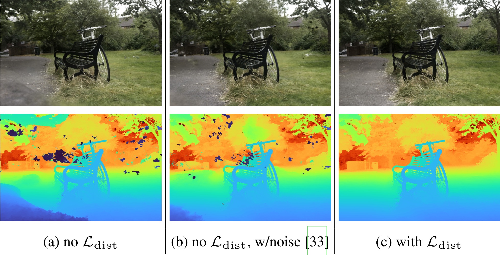
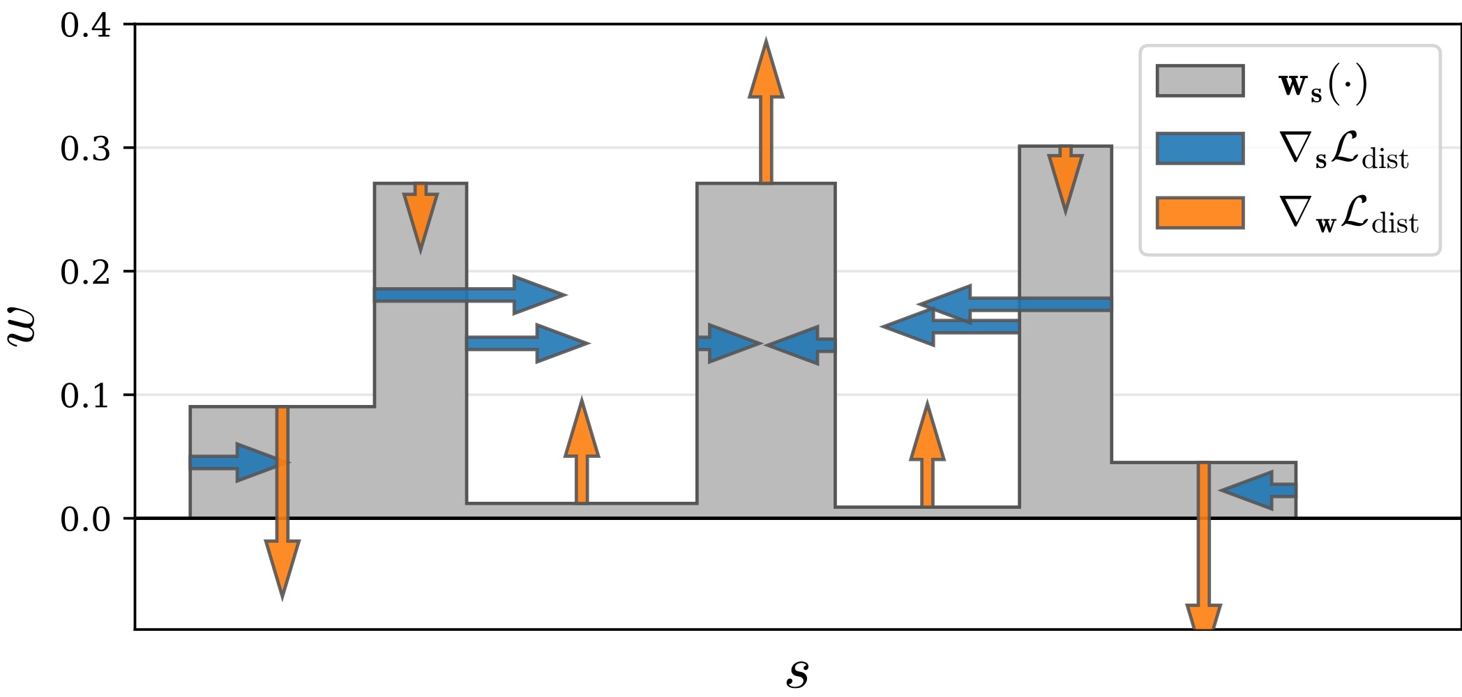
The final loss function is a combination of the reconstruction loss, the online distillation loss, and the distortion-based regularizer:

where $\lambda_{\text{prop}}$ and $\lambda_{\text{dist}}$ are hyperparameters that balance the contributions of the different loss terms. We set $\lambda_{\text{dist}} = 0.01$ and $\lambda_{\text{prop}} = 1$, as the stop-gradient ensures that the learning of the “Proposal MLP” remains independent of the “NeRF MLP.”

4.3 NeRF-W

NeRF in the Wild: Neural Radiance Fields for Unconstrained Photo Collections
CVPR 2021

NeRF in the Wild, or NeRF-W for simplicity, addresses the issue of real-world phenomena in uncontrolled, collected images, such as photometric and geometrical variations or non-static content, taken on different days or years. Applying such a dataset of images to the vanilla NeRF results in inaccurate reconstruction and severe artifacts due to its consistency assumption.

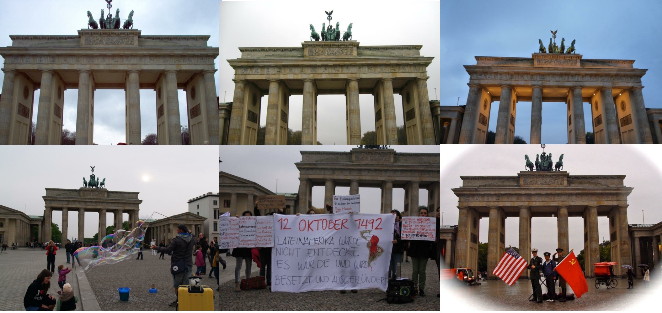
• Photometric variations: Variations caused by the time of day (day/night), atmospheric conditions (sunny/cloudy), or seasonal changes (summer/winter).
• Transient objects: Moving objects (cars, people), dynamic lighting (shadows, reflections), or other occluders.

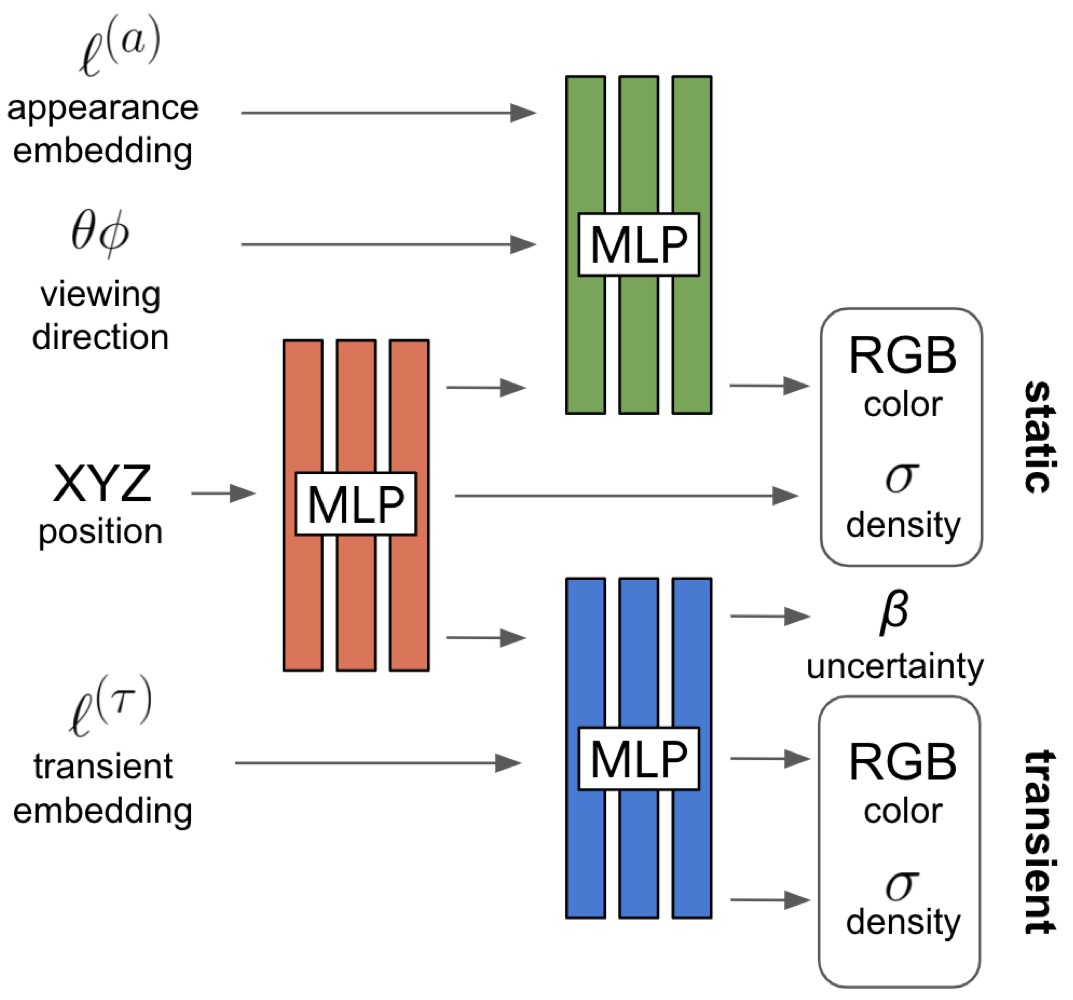
The NeRF-W model represents the volumetric density $\sigma(t)$ and color $c(t)$ using ReLU-activated MLPs as follows:

where $\gamma_x$ and $\gamma_d$ are the positional encodings of the 3D position and viewing direction, respectively. Unlike vanilla NeRF, NeRF-W’s density $\sigma(t)$ is independent of the viewing direction, while the color $c(t)$ is conditioned on the output of the first MLP $z(t)$ and the viewing direction. The NeRF-W model is trained using a collection of images ${I_i}_{i=1}^{N}$, along with their associated camera intrinsics and extrinsics.

NeRF-W proposes two enhancements to address these issues: (1) explicitly modeling the photometric variations between images and (2) estimating transient objects and disentangling them from the static scene.

Latent Appearance Modeling

NeRF-W adapts Generative Latent Optimization (GLO) to assign a latent vector $\ell_i^{(a)}$ of length $n^{(a)}$ to each image $I_i$. We can rewrite the independent color prediction as:

This extension frees NeRF from the assumption of a fixed appearance across all images by embedding illumination conditions in a smooth, continuous latent space.

Transient Object Modeling

A new “transient” head is added to NeRF-W at the color MLP level, allowing the model to reconstruct transient objects in the scene without introducing artifacts into the static scene. Without explicit supervision, the transient head learns to predict the uncertainty of each pixel in the image, allowing the reconstruction loss to ignore unreliable pixels. The Bayesian learning framework of Kendall et al. is used to model the uncertainty of the transient head.

We can rewrite the volumetric rendering equation using the static and transient color and density as:

We model $C_i(r)$ with an isotropic normal distribution with mean $\hat{C}_i(r)$ and variance $\beta_i(r)^2$, where $\beta_i(r)$ is defined as:

and the transient head MLP includes an additional input latent vector $\ell_i^{(\tau)}$, conditioned on the output of the first MLP $z(t)$:

The fine model is optimized using the negative log-likelihood of the normal distribution and an $L_1$ regularization term on the transient head:

The first two terms are the negative log-likelihood of the normal distribution of $C_i(r)$ with mean $\hat{C}_i(r)$ and variance $\beta_i(r)^2$. The third term is the $L_1$ regularization term with hyperparameter $\lambda$ on the transient density $\sigma_i^{(\tau)}(t_k)$, discouraging the transient head from reconstructing the static scene.

Together with the coarse model, which uses only the latent appearance model, we can write the total loss function for $N$ images as:

where $\mathcal{L_i}^{(c)}$ and $\mathcal{L_i}^{(f)}$ are the loss functions for the coarse and fine models, respectively.

In the next section, we will cover NeRF variants that incorporate geometric priors or supervision, primarily Depth and Point Cloud data acquired from LiDAR, Depth Sensors, or Structure-from-Motion (SfM).

These variants are designed for sparse-view NeRFs, offering faster convergence, higher quality, and requiring fewer views compared to the vanilla NeRF.

4.4 DS-NeRF

Depth-supervised NeRF: Fewer Views and Faster Training for Free
CVPR 2022

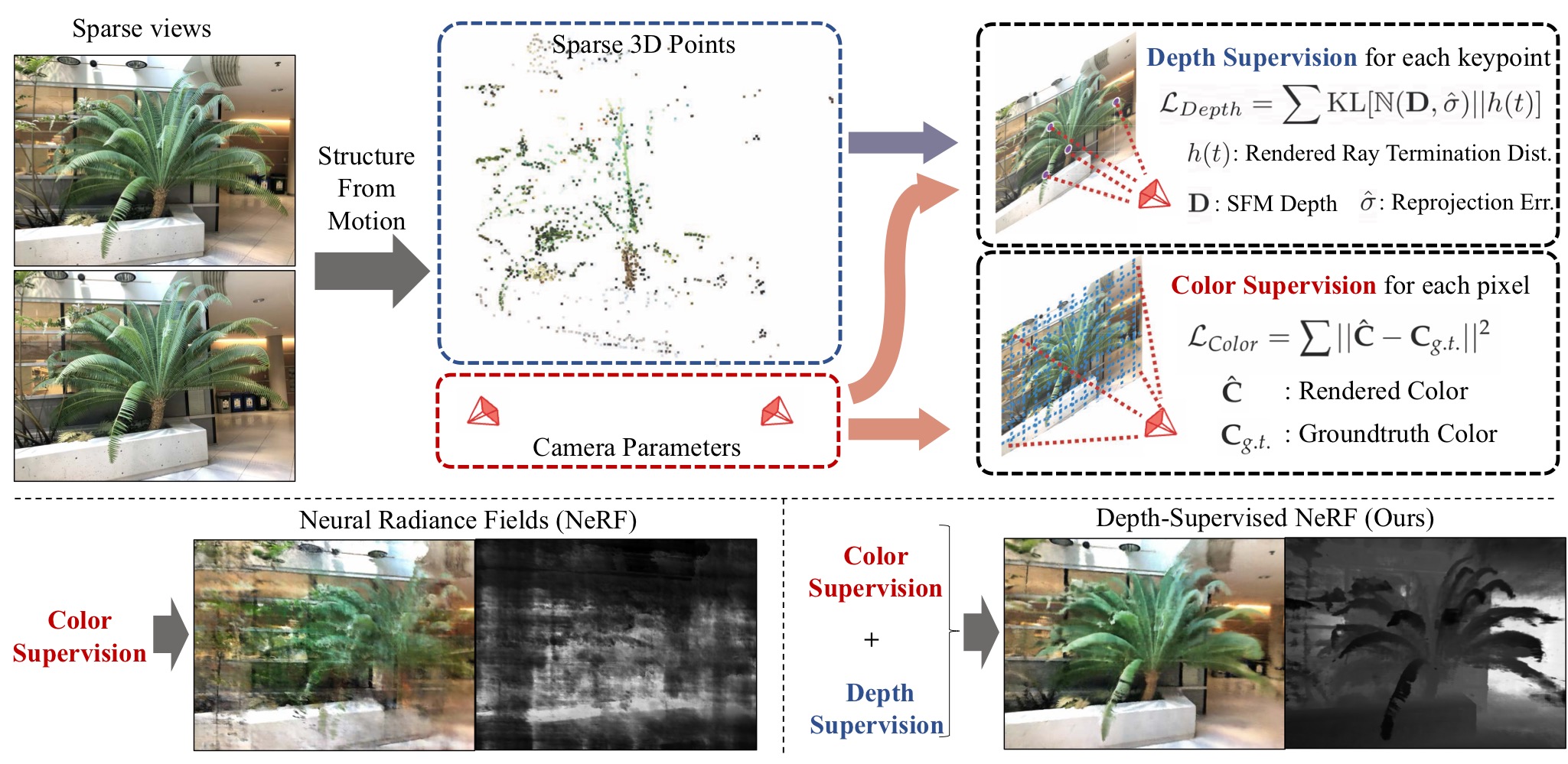
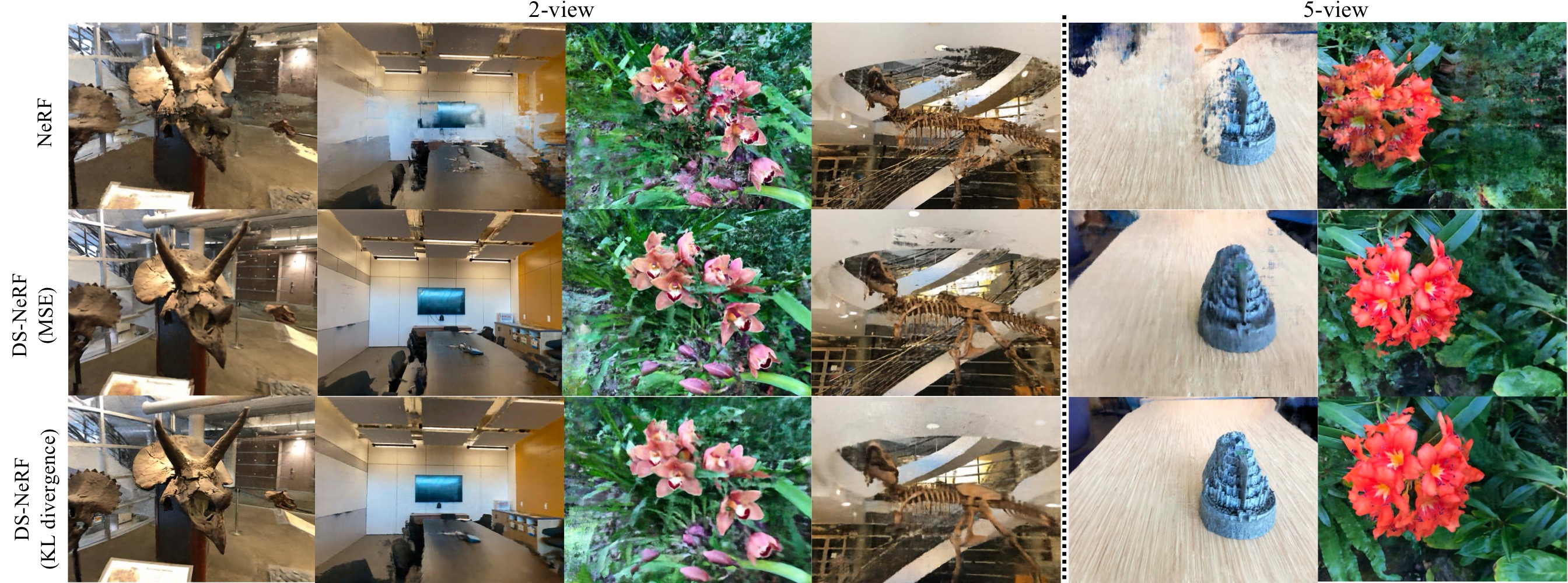
DS-NeRF addresses the issue of inconsistent geometries when fitting with fewer input views. To mitigate this, a complementary depth map or 3D point cloud from SfM or LiDAR is used to supervise the model via an additional loss term, ensuring that the termination of the ray distribution aligns with surface priors.

While NeRF produces high-quality reconstructions when using a large number of views, it can be slow due to the significant number of rays to evaluate and lengthy training times. DS-NeRF achieves better image quality with fewer training views and reduces training time by 2–3×.

• Volumetric Rendering Revisited

We recall the volumetric rendering integral for NeRF:

Let us consider $h(t) = T(t) \cdot \sigma(t)$ as a continuous probability distribution that describes the likelihood of a ray being absorbed at depth $t$, and $c(t)$ as the color at depth $t$. The ideal ray distribution for an image point with a closest surface depth of $D$ should be a Dirac delta function $\delta(t - D)$.

• Depth Supervision Modeling

Given an image $I_j$ and its camera matrix $P_j$, we estimate the depth $D_{ij}$ of visible 3D keypoints $x_i \in X_j$ by projecting them onto the image plane using the camera matrix $P_j$. The depth values $D_{ij}$ are sparse and noisy due to errors in the SfM reconstruction.

We model the depth at termination $\mathbb{D_{ij}}$ as a normal distribution around the noisy depth $D_{ij}$ with a standard deviation $\sigma_{i}$:

The objective is to minimize the KL divergence between the predicted rendering ray distribution $h(t)$ and the noisy depth distribution $\mathbb{D_{ij}}$:

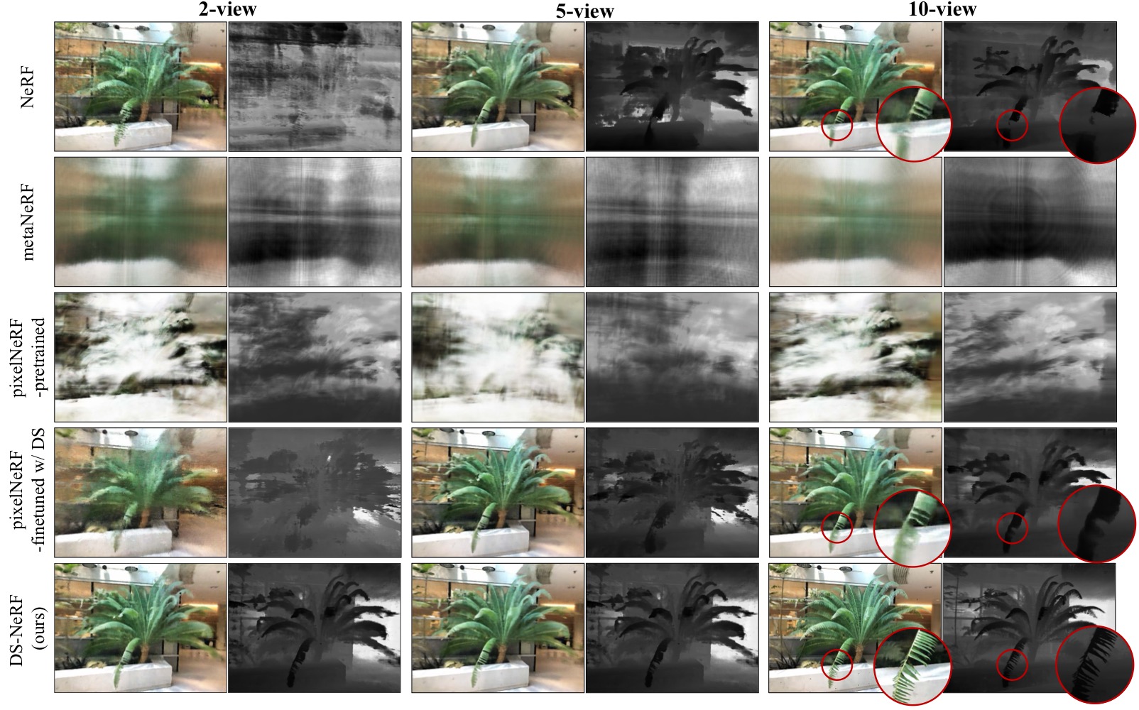
We can write the final overall reconstruction loss as:

where $\mathcal{L_{\text{color}}}$ is the color loss, $\mathcal{L_{\text{depth}}}$ is the depth supervision loss, and $\lambda_D$ is a hyperparameter that balances the two terms.

4.5 DDP-NeRF

Dense Depth Priors for Neural Radiance Fields from Sparse Input Views
CVPR 2022

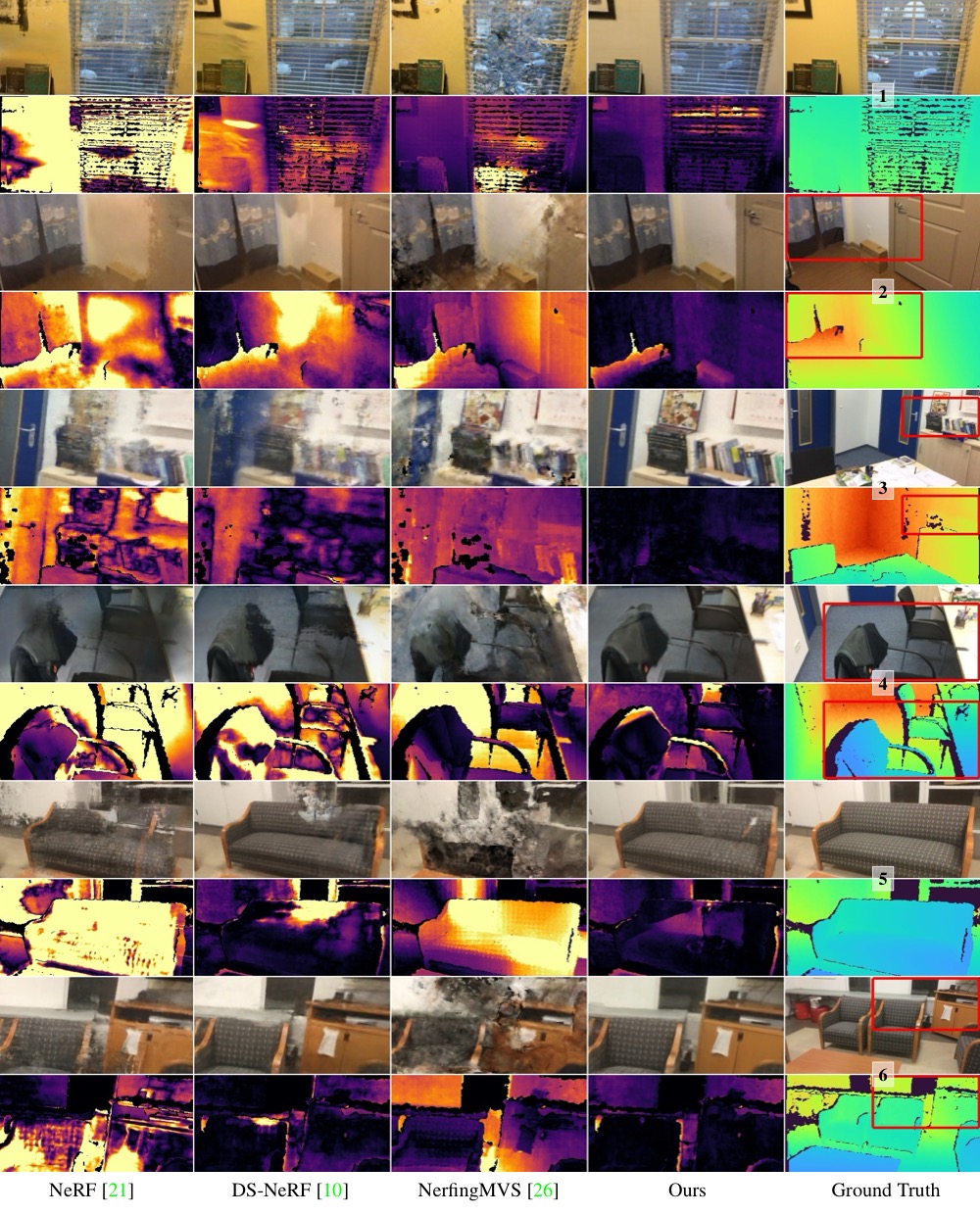
DDP-NeRF addresses the same issues as DS-NeRF by incorporating depth priors to constrain NeRF’s geometry for sparse-view reconstruction. It uses 3D points from SfM and applies depth completion to densify the depth map for supervision.

DDP-NeRF is primarily designed for indoor scenes with inside-out camera trajectories, where NeRF struggles to learn geometry due to a lack of sufficient correspondences between views, textureless flat surfaces, and appearance inconsistencies caused by lighting changes in the training images.

DDP-NeRF utilizes noisy and incomplete depth maps to produce a complete dense map and estimate an uncertainty map. This approach improves the completeness of rendered images, provides more accurate geometry, and enhances robustness to SfM outliers.

• Depth Completion with Uncertainty

Two challenges in the depth completion task are handling noisy reconstructions with outliers and the sparsity of depth maps, which varies from one image to another.

We design a depth prior network $D_{\theta_0}$ to predict dense depth maps $Z_{i}^{\text{dense}} \in [0, t_f]^{H \times W}$ with a corresponding standard deviation $S_i \in [0, \infty]^{H \times W}$ from sparse depth maps $Z_{i}^{\text{sparse}} \in [0, t_f]^{H \times W}$ and image $I_i$:

Here, $D_{\theta_0}$ is a ResNet with upsampling layers to predict the dense depth $Z_{i}^{\text{dense}}$ and the standard deviation $S_i$. For depth completion, a CSPN (Convolutional Spatial Propagation Network) is employed in each branch to refine the depth map, making it more detailed and accurate by propagating information from neighboring pixels over iterations.

• Depth Supervision

DDP-NeRF is trained using sampled depths at sparse points, perturbed using a Gaussian distribution $\mathcal{N}(0, s_{\text{noise}}(z)^2)$, where the standard deviation $s_{\text{noise}}(z)$ increases with depth $z$ to account for depth uncertainty. The depth supervision loss is defined as:

where $n$ is the number of sparse points, $z_j$ is the noisy depth, $z_j^{\text{dense}}$ is the dense depth, and $s_j$ is the standard deviation.

• NeRF with Dense Depth Priors

Inspired by NeRF-W, DDP-NeRF uses an additional input to the network with an image embedding vector $\ell_i^{(a)}$ to predict the density $\sigma_i(t)$ and the color $c_i(t)$ under appearance inconsistencies in the captured images:

In addition to the predicted color, a NeRF depth estimate $\hat{z}(r)$ and standard deviation $s(r)$ are used to supervise the radiance field according to the learned depth prior. The depth estimate and standard deviation are defined as:

The NeRF parameters $\theta_1$ are optimized using the following loss function $\mathcal{L_{\theta_1}}$:

where:

with:

Here, $z(r)$ and $s(r)$ are the noisy depth and the standard deviation, obtained from the corresponding $Z_i^{\text{dense}}$ and $S_i$ maps.

This loss encourages NeRF to terminate rays within a standard deviation at the most certain depth prior while allocating density to minimize the color loss.

• Depth-Guided Sampling

Depth is used to guide the sampling process in DDP-NeRF. Half of the samples follow the near-to-far sampling strategy, while the other half follow a Gaussian distribution around the depth prior $\mathcal{N}(z(r), s(r)^2)$.

NerfingMVS

PointNeRF

Adjusent to Neural Rendreing

4.6 Plenoxels

Plenoxels: Radiance Fields without Neural Networks
CVPR 2022

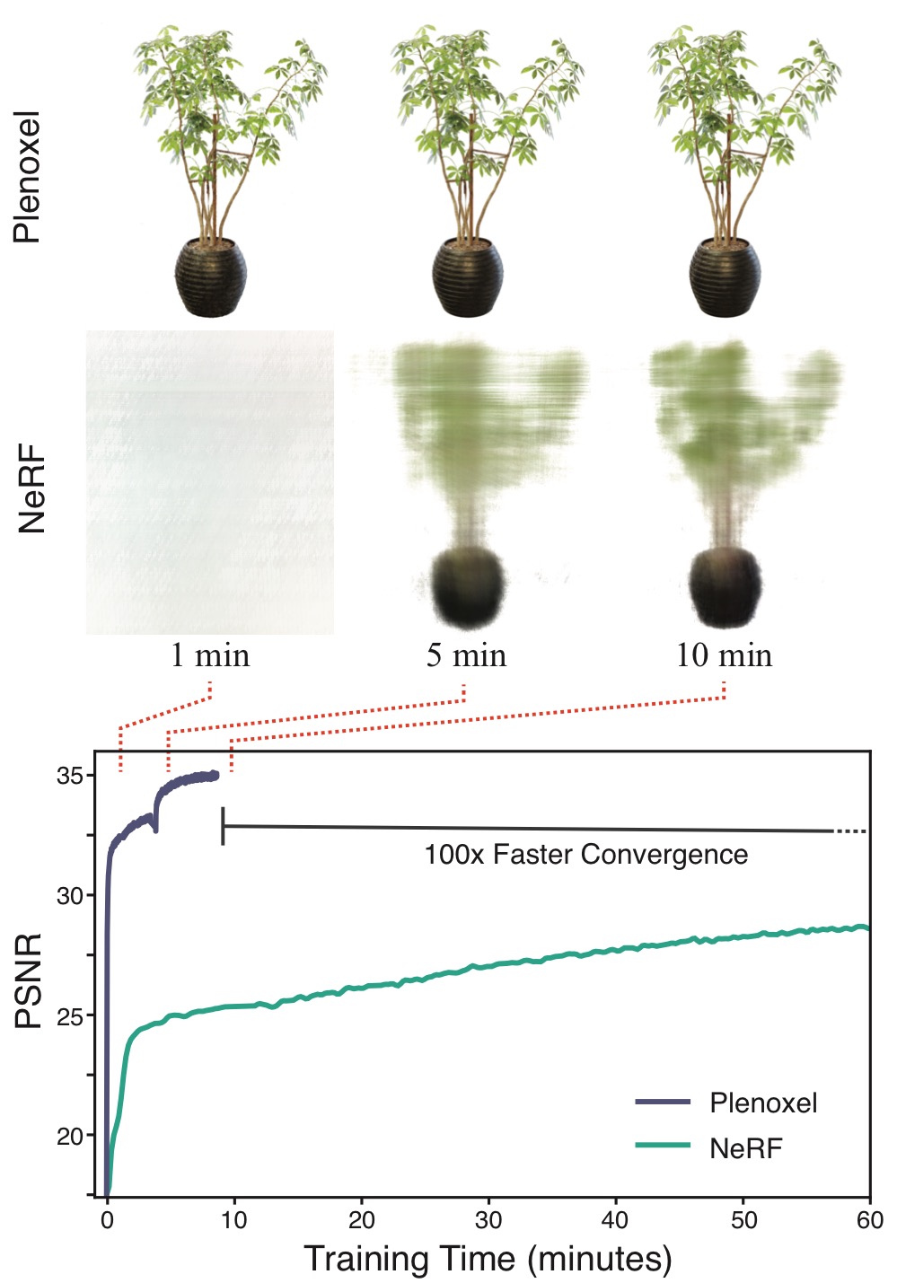
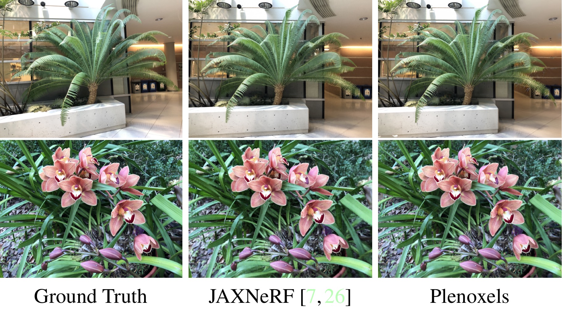
Plenoxels is a novel approach to radiance fields that replaces neural networks with a sparse 3D voxel grid augmented by spherical harmonics for view-dependent effects. This explicit representation achieves rendering speeds of 15 fps and training times two orders of magnitude faster than NeRF, while maintaining comparable reconstruction quality.

Each voxel stores opacity and spherical harmonics coefficients, encoding density and color information. Empty voxels are pruned to optimize storage, and octree structures enable memory efficiency and adaptive resolution. Trilinear interpolation ensures smooth transitions, and a coarse-to-fine optimization strategy refines high-resolution reconstructions.

Plenoxels are optimized using a differentiable rendering loss with total variation regularization to reduce noise and enforce smoothness. By directly optimizing voxel parameters through forward volume rendering, Plenoxels avoid neural-network pipelines.

As a generalization of PlenOctrees, Plenoxels support arbitrary-resolution voxel grids with spherical harmonics, offering a fast and scalable alternative to neural-network-based radiance fields.

• Voxel Grid and Spherical Harmonics

Plenoxels use a dense 3D index array pointing to a data array that stores values only for occupied voxels, eliminating the need for an octree structure and enabling faster access and simpler memory management.

Each occupied voxel encodes a scalar opacity value ($\sigma$) and spherical harmonics (SH) coefficients for the color channels. Using degree-2 spherical harmonics, Plenoxels store 9 coefficients per color channel, totaling 27 coefficients per voxel.

Trilinear interpolation is applied to ensure smooth transitions, defining a continuous plenoptic function and improving upon the constant-coefficient assumption of PlenOctrees.

• Interpolation & Coarse-to-Fine

Trilinear interpolation computes the opacity and color at sample points using harmonic coefficients from the 8 nearest voxels, providing a continuous function, which improves optimization stability.

The coarse-to-fine strategy begins with a low-resolution voxel grid, optimizes it, prunes unnecessary voxels, and refines by subdividing each voxel. Grids start at $256^3$ and upscale to $512^3$, with trilinear interpolation ensuring smooth transitions and detail preservation.

Voxel pruning, based on thresholds for voxel weights or density, is enhanced by a dilation operation to prevent issues near surfaces. This ensures that only unoccupied voxels and their neighbors are removed.

• Optimization & Regularization

Plenoxels are optimized using reconstruction and TV regularization losses, minimizing the difference between rendered and ground-truth images while enforcing smoothness:

Where:

with $\Delta_x^2(v,d)$, $\Delta_y^2(v,d)$, and $\Delta_z^2(v,d)$ representing the squared differences in voxel values along the $x$, $y$, and $z$ axes, respectively.

The problem is challenging due to its non-convex rendering function; thus, RMSprop is used to optimize voxel parameters.

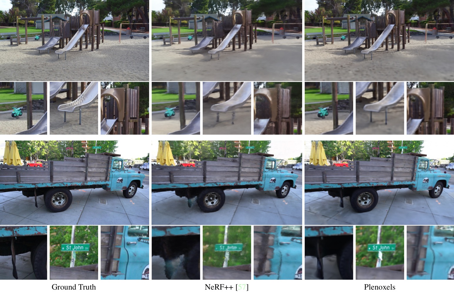
Plenoxels achieve good results for a wide range of settings, including real unbounded scenes, 360° and forward-facing cameras. Additional regularization terms include a sparsity prior based on a Cauchy loss as follows:

where $\sigma(r_i(t_k))$ is the opacity of the voxel at the ray $r_i$ of sample $k$.

For 360° scenes, a beta distribution regularization term is applied to the accumulated foreground of each ray, encouraging the foreground to be fully opaque:

where $T_{FG}(r)$ is the accumulated foreground opacity of the ray $r$ between 0 and 1.

TensoRF

Non-Backed

Instant Neural Graphics Primitives Instant-NGP

Large Scale

Block-NeRF

Reg-NeRF

TODO: Review the DONeRF for smapling orackle networks and TermiNeRF