A Comprehensive Study for Gaussian Splatting
Published:
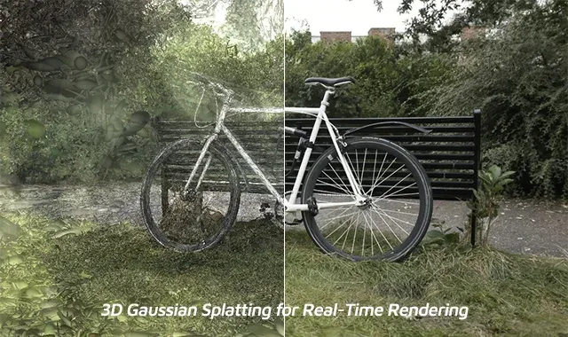
Gaussian Splatting is a cutting edge technique for real time neural rendering that models scenes using explicit 3D Gaussians. It offers an alternative to neural implicit representations (NIR) and NeRFs. This study provides a rigorous, structured exploration of its mathematical foundations, differentiable rasterization pipeline, and key advancements that are redefining Gaussian-based scene representation.
Table of Contents
- Introduction
- 3D Gaussian Representation
2.1 Point-Based Rendering
2.2 Scene Representation with Splats - Optimization and Adaptive Density Control 3.1 Optimization of Gaussian Parameters
3.2 Adaptive Density Control - Differentiable Tile-Based Rasterization
- Training Pipeline
- View-Dependent Colors with Spherical Harmonics
- Final Remarks
7.1 Comparison with NeRF
7.2 Applications - References
- Appendix: Code Snippets
1. Introduction
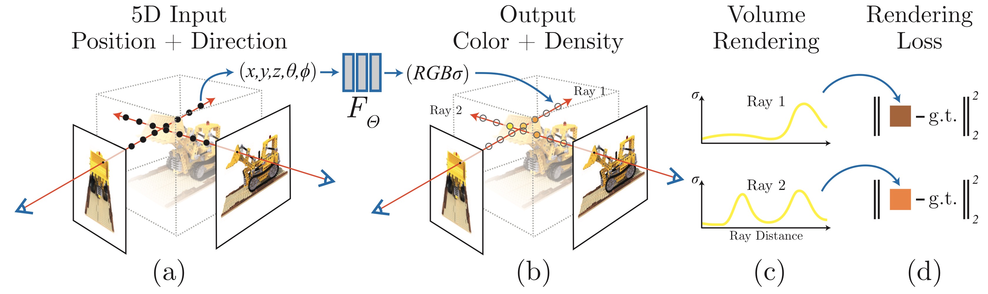
Gaussian Splatting (GS) is a recent breakthrough in real-time neural rendering that represents 3D scenes as unstructured sets of anisotropic Gaussian ellipsoids. In contrast to NeRFs, which rely on implicit volumetric representations encoded by multi-layer perceptrons (MLPs), GS employs an explicit, differentiable formulation that supports efficient rasterization and fast convergence.
While NeRF and its variants have achieved impressive photorealism in novel view synthesis, they exhibit notable limitations: slow training and inference, high memory usage, and inefficiencies in modeling empty space. Gaussian Splatting addresses these challenges through:
- Explicit 3D Gaussians for spatial representation
- Alpha compositing and spherical harmonics for view-dependent appearance
- Tile-based differentiable rasterization for real-time performance on modern GPUs
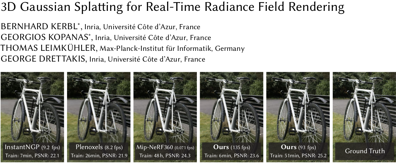
Introduced by Kerbl et al., 2023, Gaussian Splatting replaces neural field representations with a compact, interpretable formulation that enables fast optimization, real-time rendering, and high-fidelity view synthesis.
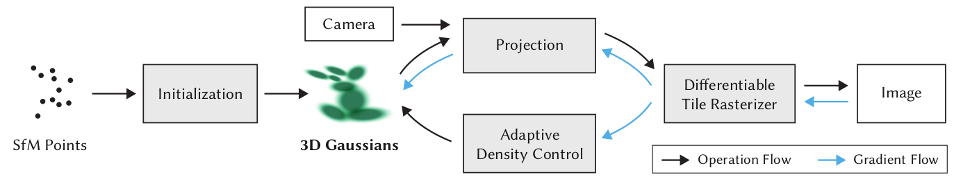
2. 3D Gaussian Representation
3D Gaussian Splatting is a real-time rendering method that represents scenes using millions of Gaussian primitives instead of triangles. Starting from a sparse SfM point cloud and calibrated cameras, Gaussians are optimized with adaptive density control to refine their placement and appearance. A fast, differentiable tile-based rasterizer then enables high-quality rendering with competitive training times, supporting interactive exploration of photorealistic 3D scenes.
We begin with a brief overview of point-based rendering, then detail the Gaussian Splatting pipeline, including scene representation, rasterization, and optimization.
2.1 Point-Based Rendering
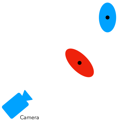
In this paradigm, a 3D scene is modeled as a set of discrete spatial primitives such as particles, surfels, or ellipsoids. These points are projected onto the image plane and blended to form continuous surfaces and radiance fields in screen space.
Classical point-based methods rely on simple splatting of fixed radius points, which often leads to visual artifacts such as aliasing, discontinuities, and poor reconstruction of view dependent effects.
To address these issues, modern techniques introduce several enhancements, including:
- Anisotropic splats that align with surface geometry and adapt their shape per viewpoint.
- Opacity-aware alpha blending to simulate volumetric transmittance and occlusion.
- Spherical Harmonics (SH) to encode view-dependent appearance.
Let \(\mathcal{G} = {g_i}_{i=1}^N\) denote a set of \(N\) point primitives, where each \(g_i\) is defined by parameters \((\mu_i, \Sigma_i, \alpha_i, c_i, SH_i)\). The rendered pixel color \(C\) along a camera ray \(\mathbf{r}\) is computed via front-to-back alpha compositing:
\[C(\mathbf{r}) = \sum_{i=1}^N T_i \alpha_i c_i \quad \text{where} \quad T_i = \prod_{j=1}^{i-1} (1 - \alpha_j)\]This formulation is mathematically equivalent to the volumetric rendering equation used in NeRF, but instead of stochastic sampling in a continuous field, it operates on projected 2D Gaussian splats.
2.2 Scene Representation with Splats
Each point in the scene is modeled as a 3D anisotropic Gaussian, which is differentiable and can be efficiently projected into 2D splats for rasterization. However, Structure-from-Motion (SfM) point clouds are often sparse and lack reliable surface normals (noisy), making direct surface modeling difficult.
To address this, each Gaussian is defined by a 3D covariance matrix \(\Sigma_i\) in world space, centered at its mean position \(\mu_i\). The spatial influence of a Gaussian is given by:
\[G_i(\mathbf{x}) = \sigma({\alpha}) \exp\left(-\frac{1}{2}(\mathbf{x} - \mu_i)^T \Sigma_i^{-1} (\mathbf{x} - \mu_i)\right)\]where \(\mathbf{x} \in \mathbb{R}^3\) is a query point in 3D space. \(\alpha\) is a scaling factor that controls the Gaussian’s opacity, and \(\sigma(\alpha)\) is a function that maps the opacity to a suitable range.
🧭 Projection to Camera Space:
To project a 3D Gaussian into 2D, we use the camera projection matrix \(P = [R \mid t]\), where:
- \(R\) is the camera rotation matrix
- \(t\) is the camera translation vector
The Gaussian mean and covariance transform as:
\(\mu_{\text{camera}, i} = R \cdot \mu_i + t\) \(\Sigma_{\text{camera}, i} = R \cdot \Sigma_i \cdot R^T\)
So the projected Gaussian in camera coordinates becomes:
\[\mathcal{N}(\mu_{\text{camera}, i}, \Sigma_{\text{camera}, i})\]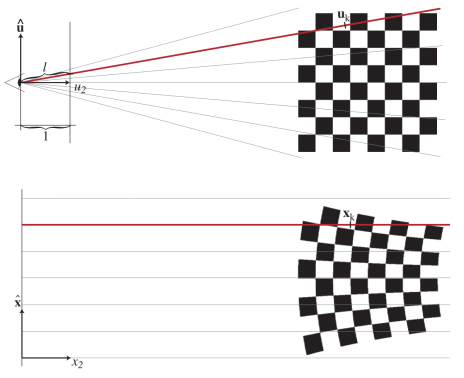
📡 Ray Space Transformation:
Rather than immediately projecting into 2D, the system introduces an intermediate Ray Space, as proposed in the EWA Volume Splatting paper. In this coordinate system, rays are aligned parallel to an axis, making it easier to analytically integrate over the splat without sampling along the ray (unlike NeRF).
To transform into Ray Space, we apply the Jacobian \(J_i\) of the projection function at \(\mu_{\text{camera}, i}\):
\[\Sigma_{\text{ray}, i} = J_i \Sigma_{\text{camera}, i} J_i^T = J_i R \Sigma_i R^T J_i^T\]This transformation warps the Gaussian to match how it appears along a ray-aligned coordinate system while preserving symmetry.
Zwicker’s paper shows that if we skip the third row and column of the covariance matrix, we obtain a \(2 \times 2\) covariance matrix suitable for 2D splatting. This simplification effectively slices the ellipsoid along the viewing direction, producing a 2D elliptical footprint in Ray Space that preserves the key anisotropic properties of the original \(3 \times 3\) covariance—just as if we had started from planar points with known normals.
However, transforming and optimizing these Gaussians requires care, as covariance matrices must have physical meaning. Covariance matrices must remain positive semi-definite (PSD) to be valid, meaning all eigenvalues must be non-negative. Directly optimizing \(\Sigma_i\) using gradient descent can easily violate this constraint, especially when updates push the matrix toward singular or indefinite configurations.
To preserve PSD structure during training, the authors reparameterize each 3D covariance matrix as an ellipsoid:
\[\Sigma_i = R_i S_i S_i^T R_i^T\]Here:
- \(S_i\) is a diagonal matrix of non-negative scale values, encoding the lengths of the ellipsoid’s principal axes.
- \(R_i\) is a rotation matrix constructed from a normalized quaternion \(q\) determining the orientation of the ellipsoid in 3D space.
This factorization ensures that \(\Sigma_i\) is always symmetric and PSD by construction. It also separates geometry into interpretable components: Scale and Orientation.
By operating in this ray-aligned space, the splatting process avoids the need for discrete point sampling along rays—as is required in NeRF—and instead enables efficient, closed-form rasterization of these warped ellipsoids.
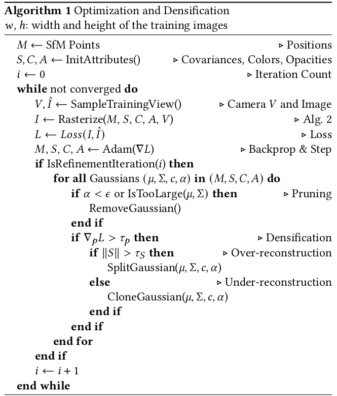
3. Optimization and Adaptive Density Control
The optimization pipeline in 3D Gaussian Splatting jointly refines scene geometry and appearance by updating each Gaussian’s parameters through supervised rendering loss.
It consists of two core components: The Optimization of Gaussian Parameters and an Adaptive Density Control.
3.1 Optimization of Gaussian Parameters
The optimization is driven by comparing rendered images against ground-truth views. For a sampled camera \(P_k\) and its corresponding image \(I_k\), the system renders an image \(\hat{I}_k\) using the current set of Gaussians projected into view space.
A differentiable loss is then computed, composed of two terms: a photometric \(L_1\) loss and a perceptual \(L_{\text{D-SSIM}}\) loss:
\[\mathcal{L}(I_k, \hat{I}_k) = (1 - \lambda) \cdot \| I_k - \hat{I}_k \|_1 + \lambda \cdot \mathcal{L}_{\text{D-SSIM}}(I_k, \hat{I}_k)\]- \(\lambda\) is a weighting factor (typically set to 0.2) that balances the contribution of the two loss terms.
- \(\mathcal{L}_{\text{D-SSIM}}\) is the Differentiable Structural Similarity Index loss, which encourages alignment in luminance, contrast, and structural features between \(I_k\) and \(\hat{I}_k\).
The SSIM-based term is defined as:
\[\mathcal{L}_{\text{D-SSIM}} = 1 - SSIM(x, y)\]where \(x\) and \(y\) are patches from the rendered and ground-truth images. SSIM considers local statistics:
- \(\mu_x\), \(\mu_y\): local means
- \(\sigma_x^2\), \(\sigma_y^2\): variances
- \(\sigma_{xy}\): covariance
- \(c_1 = (k_1 L)^2\), \(c_2 = (k_2 L)^2\) stabilize division, with \(k_1 = 0.01\), \(k_2 = 0.03\), and \(L\) the dynamic range
The optimizer used is Adam, and gradients are computed and backpropagated through the rendering pipeline to update four key learnable parameters for each Gaussian:
- Position \(\mu_i\)
- Covariance \(\Sigma_i = R_i S_i S_i^T R_i^T\)
- Color coefficients \(c_i\) (via spherical harmonics \(SH_i\))
- Opacity \(\alpha_i\)
Since the covariance matrix \(\Sigma_i\) is parameterized by a rotation \(R_i\) (from a quaternion \(q\)) and scale \(S_i\), the gradients are computed indirectly:
\[\frac{\partial \mathcal{L}}{\partial s}, \quad \frac{\partial \mathcal{L}}{\partial q}\]This allows the system to perform stable and efficient updates while preserving the positive semi-definite property of the covariance.
3.2 Adaptive Density Control
While optimizing parameters improves accuracy, maintaining an effective Gaussian distribution requires dynamic adaptation of their count and placement.
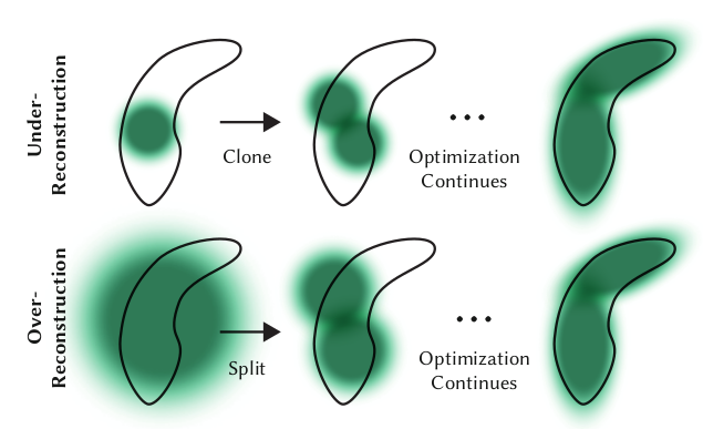
The density control loop periodically adjusts the Gaussian set with three operations:
Cloning: Gaussians with high position gradient magnitude are duplicated and shifted to improve coverage in under-represented areas.
Splitting: Gaussians with large spatial extent or covering high-frequency details are split into two smaller Gaussians:
\(\Sigma_i \rightarrow \Sigma_i^{(1)}, \Sigma_i^{(2)}, \quad s^{(j)} = \frac{1}{\phi} s_i\) where \(\phi > 1\) is a shrink factor (typically 1.6), and the new means are sampled from the original Gaussian’s PDF.Pruning: Gaussians are removed if:
- \(\alpha_i < \epsilon_{\alpha}\) (opacity threshold) for transparency
- They have excessively large footprints (in world or image space)
This densification/pruning is run every few hundred iterations (e.g., every 100 steps), ensuring that the model:
- Adds detail where needed
- Keeps parameter count efficient
- Prevents under-reconstruction and over-reconstruction regions.
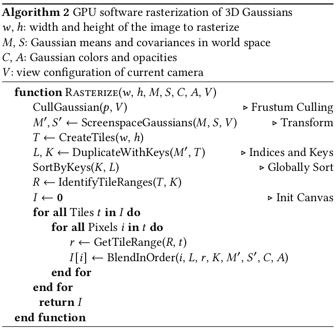
4. Differentiable Tile-Based Rasterization
To enable real-time rendering and end-to-end optimization, 3D Gaussian Splatting employs a fully differentiable, tile-based rasterizer. Below we outline its key steps:
Step 1: Cull Gaussians Outside the View Frustum
For each Gaussian \(g_i\) with mean \(\mu_i\) and 99% confidence interval, we discard it if:
- \(\mu_i\) is outside the frustum depth range \(z_{\text{near}} < z_i < z_{\text{far}}\)
- The confidence region does not intersect any visible area
- It lies within a guard band near the near/far planes
Function: CullGaussian(\(\mu_i\), \(P\))
Step 2: Project to Screen Space
For each surviving Gaussian, compute:
Screen-space mean: \(\mu_i' = \pi(R \mu_i + t)\)
Ray-space covariance: \(\Sigma_{\text{ray}, i} = J_i \cdot R \Sigma_i R^T \cdot J_i^T\)
where \(J_i\) is the Jacobian of the projection function at \(\mu_i\).
Function: ScreenspaceGaussians(\(\mu_i\), \(\Sigma_i\), \(P\))
Step 3: Create Screen Tiles
Divide the screen into \(T = \lceil w/16 \rceil \times \lceil h/16 \rceil\) tiles of \(16 \times 16\) pixels.
This enables efficient parallel GPU processing.
Function: CreateTiles(w, h)
Step 4: Duplicate Gaussians per Tile
Each Gaussian’s projected 2D footprint (ellipse) may span multiple screen tiles.
To ensure full coverage, we duplicate the Gaussian for every tile it overlaps.
Function: DuplicateWithKeys(\(M’\), \(T\))
Step 5: Assign Sorting Keys and Sort Duplicates
Each duplicated Gaussian is assigned a sorting key that encodes:
- Its tile ID (indicating which tile it affects)
- Its view-space depth (for visibility ordering)
The full list of duplicates is then globally sorted using GPU Radix Sort. This ensures that within each tile, Gaussians are composited in front-to-back order.
Function: SortByKeys(\(K\), \(L\))
Step 6: Identify Per-Tile Gaussian Ranges
Determine index ranges \([s_j, e_j]\) in the sorted list for each tile \(t_j\).
Function: IdentifyTileRanges(T, K)
Step 7: Rasterize Each Tile in Parallel
Each GPU thread block processes one tile:
- Load Gaussians in range \([s_j, e_j]\) into shared memory.
- For each pixel \(p\):
- Blend Gaussians front-to-back using: \(C_p = \sum_n T_n \alpha_n c_n, \quad T_n = \prod_{m < n}(1 - \alpha_m)\)
- Stop when total opacity saturates: \(\sum \alpha_n \geq 1\)
Function: RasterizeTile(tile_id, [s_j, e_j])
To enable backpropagation, the final accumulated opacity \(\alpha_{\text{accum}}\) is stored during the forward pass.
In the backward pass, Gaussians are traversed in reverse, and transmittance is recovered via:
This avoids storing full blending chains and allows efficient gradient computation for all contributing Gaussians.
5. Training Pipeline
The training process for 3D Gaussian Splatting optimizes scene representation by minimizing the photometric discrepancy between rendered and ground-truth images. It is fully differentiable and GPU-accelerated, enabling fast convergence compared to implicit methods like NeRF.
Initialization:
We start with a sparse SfM point cloud and calibrated camera poses.
- SfM-based point cloud: Provides initial 3D positions and calibrated camera poses using COLMAP for structure-from-motion.
- Gaussian parameters: Each point is initialized with Position \(\mu_i\), Isotropic covariance \(\Sigma_i = \sigma^2 I\), View-independent color \(c_i\) and Opacity \(\alpha_i\)
These parameters are then optimized through a series of training iterations.
Differentiable Rendering:
In the forward pass, and for each camera view with its corresponding image, the following steps are performed:
- Cull Gaussians outside the camera frustum.
- Project Gaussians to 2D screen space using camera matrices and Jacobians.
- Rasterize using tile-based GPU sorting and front-to-back alpha blending.
Compose output image using:
\[C(\mathbf{r}) = \sum_i T_i \alpha_i c_i, \quad T_i = \prod_{j=1}^{i-1} (1 - \alpha_j)\]
Optimization:
We compute the loss between the rendered image and the ground truth image using a composite loss function, where \(\lambda\) is typically 0.2: \(\mathcal{L}(I_{\text{gt}}, I_{\text{pred}}) = (1 - \lambda) \|I_{\text{gt}} - I_{\text{pred}}\|_1 + \lambda \cdot \mathcal{L}_{\text{D-SSIM}}\)
In the backwards pass, we use the Adam optimizer to update the learnable parameters of the Gaussians.
Densification and Pruning:
Every few hundred iterations, we perform a densification and pruning step to adaptively control the Gaussian set via {Clone, Split, Prune} operations.
6. View-Dependent Colors with Spherical Harmonics
To make a 3D scene look realistic, surface colors must change based on the viewing angle. For example, shiny objects often appear brighter or darker depending on where the camera is positioned. Gaussian Splatting captures this effect by assigning each point a color that varies with the view direction.
Unlike NeRF, which relies on a heavy neural network to learn appearance, Gaussian Splatting uses a lightweight and efficient technique called spherical harmonics (SH). Each point stores a compact set of SH coefficients that describe how its color should change when viewed from different angles. This representation is fast to evaluate and requires far less computation than NeRF’s multi-layer perceptrons.
Spherical harmonics are widely used in graphics for representing directional lighting, ambient occlusion, and precomputed radiance transfer. Their ability to approximate smooth angular functions with just a few coefficients makes them ideal for real-time rendering tasks. For a deeper dive into SH and its applications in rendering, see Green, 2003 – Spherical Harmonic Lighting: The Gritty Details.
7. Final Remarks
3D Gaussian Splatting (3DGS) offers a practical and high-performance alternative to NeRFs by representing 3D scenes with millions of explicit Gaussian primitives. It stands out for its efficiency, simplicity, and real-time capabilities:
No Neural Networks: 3DGS avoids deep learning entirely, relying on direct optimization and tile-based rasterization to achieve real-time performance (~30 FPS on a single GPU).
Compact Scene Encoding: Each Gaussian encodes position, shape (via covariance), opacity, color, and view-dependent appearance using spherical harmonics.
Fast and Stable Training: Optimization uses a combination of L1 and D-SSIM loss, with adaptive density control through cloning, splitting, and pruning of Gaussians.
Real-Time Rendering: Tile-based GPU rasterization enables high-resolution, real-time rendering through parallel compositing of sorted Gaussian splats.
Efficient View-Dependence: Spherical harmonics provide a lightweight way to model color variation with viewing direction—without the cost of a neural network.
However, 3DGS also comes with a few practical trade-offs:
Large File Sizes: Final
.plyoutputs can range from 100–200 MB due to the large number of Gaussians and associated parameters.Full View Coverage Required: High-quality reconstruction demands image capture from all angles. Missing views can lead to incomplete or biased results.
Specialized Viewers Needed: Standard 3D viewers do not fully support Gaussian-enhanced
.plyfiles. Tools like SuperSplat, Splatviz, Viser, and Three.js visualizers are required for proper inspection or editing.No Native Mesh Output: 3DGS does not produce meshes. To generate surfaces, external tools like SuGaR (Surface-Aligned Gaussian Splatting) must be used.
7.1 Comparison with NeRF
| Feature | 3D Gaussian Splatting (3DGS) | Neural Radiance Fields (NeRF) |
|---|---|---|
| Representation | Explicit 3D Gaussians | Implicit MLP (Neural Field) |
| Rendering | Tile-based rasterization | Volumetric ray marching |
| Training Time | Minutes | Hours to days |
| Inference Speed | Real-time (30+ FPS) | Slow (1–5 FPS) |
| View-Dependence | Spherical Harmonics | Learned via MLP |
| Neural Network | ✗ None | ✓ Required |
7.2 Applications
3D Gaussian Splatting represents a major leap in real-time neural rendering. By combining explicit geometry, efficient GPU pipelines, and fast training, it delivers photorealistic results without the complexity of deep networks.
Its strengths make it especially well-suited for a range of real-time 3D applications, including:
- Augmented and Virtual Reality (AR/VR): Fast inference and compact scene representation support immersive, low-latency environments.
- Gaming: Real-time rendering with dynamic viewpoints and high visual fidelity, without the overhead of large neural models.
- Digital Twins and Simulation: Accurate spatial reconstructions with real-time navigation and visualization.
- 3D Web and Mobile Experiences: Rendered directly in-browser using lightweight viewers like Three.js or gSplats.
- Interactive Content Creation: Enables creators to reconstruct and edit real-world scenes quickly with visual feedback.
With growing community support and open-source tooling, 3DGS is rapidly becoming a practical, scalable alternative to neural fields for production-level 3D graphics.
8. References
Papers:
- Kerbl et al., 2023: 3D Gaussian Splatting for Real-Time Radiance Field Rendering.
- Green, 2003: Spherical Harmonic Lighting: The Gritty Details.
- Zwicker et al., 2001: EWA Volume Splatting.
- Memory-Efficient 3DGS, 2024: Reducing the Memory Footprint of 3D Gaussian Splatting.
Blogs & Tutorials:
- LearnOpenCV: 3D Gaussian Splatting Explained.
- PyImageSearch, 2024: 3D Gaussian Splatting vs NeRF: The End Game of 3D Reconstruction.
Code & Resources:
- Graphdeco GitHub: Official 3D Gaussian Splatting Implementation.
- Awesome 3D Gaussian Splatting: Curated list of papers, tools, and resources.
Appendix: Code Snippets
The following code snippets capture the core implementation details of 3D Gaussian Splatting. Each section corresponds to a key stage in the pipeline: training, densification, and tile-based rasterization.
Training Loop:
Trainer:
  # Training options and parameters
  opt = {
      "iterations": 100000,              # Total number of training steps
      "optimizer_type": "adam",          # Optimizer choice adam or sparse_adam
      "lambda_dssim": 0.2,               # Weight for D-SSIM in the loss function
      "depth_l1_weight_init": 0.1,       # Weight for inverse depth supervision
      "densify_until_iter": 50000,       # Stop densifying halfway through training
      "densification_interval": 100,     # How often to perform clone/split/prune
  }

  def training(dataset, **kwargs):
      # Initialize model and scene
      gaussians = GaussianModel(dataset.sh_degree, opt["optimizer_type"])
      scene = Scene(dataset, gaussians)
      gaussians.training_setup(opt)

      # Background color used during training
      background = torch.tensor(
          [1, 1, 1] if dataset.white_background else [0, 0, 0], device="cuda"
      )

      # -> Start training loopu
      for iteration in range(opt["iterations"]):
          gaussians.update_learning_rate(iteration)

          # Gradually increase SH degree during training
          if iteration % 1000 == 0:
              gaussians.oneupSHdegree()

          # Sample a random training camera
          viewpoint_cam = random.choice(scene.getTrainCameras())

          # Render from current Gaussian state
          render_results = render(viewpoint_cam, gaussians, background, **kwargs)
          image = render_results["image"]
          image_gt = viewpoint_cam.original_image.cuda()  # Original image

          # Photometric loss (L1 + SSIM)
          l1_loss_val = l1_loss(image, image_gt)
          ssim_loss_val = ssim(image, image_gt)
          loss = (1 - opt["lambda_dssim"]) * l1_loss_val + opt["lambda_dssim"] * (1 - ssim_loss_val)

          # Optional depth supervision (inverse depth map)
          if viewpoint_cam.depth_reliable:
              inv_depth_pred = render_results["depth"]
              inv_depth_gt = viewpoint_cam.invdepthmap.cuda()
              depth_mask = viewpoint_cam.depth_mask.cuda()

              # Compute masked L1 loss in inverse depth
              depth_l1 = torch.abs((inv_depth_pred - inv_depth_gt) * depth_mask).mean()
              loss += opt["depth_l1_weight_init"] * depth_l1  # Update the loss

          # Backpropagation and update Gaussian parameters
          loss.backward()
          gaussians.optimizer.step()
          gaussians.optimizer.zero_grad(set_to_none=True)

          # Density Control, Clone/split/prune Gaussians to adapt to scene geometry
          if iteration < opt["densify_until_iter"] and iteration % opt["densification_interval"] == 0:
              gaussians.densify_and_prune(...)

      # Save the final trained model
      torch.save(gaussians.capture(), f"{scene.model_path}/final.pth")
L1 Loss:
The L1 loss measures pixel-wise absolute differences between the rendered and ground-truth images. It encourages color accuracy and penalizes intensity mismatches
  def l1_loss(network_output, gt):
    # Mean absolute error over all pixels
    return torch.abs(network_output - gt).mean()
SSIM Loss:
SSIM (Structural Similarity Index Measure) evaluates structural similarity based on local statistics (mean, variance, covariance) over patches. It helps preserve texture, edges, and high-frequency content.
  def create_window(window_size, channel):
      # Create a 2D Gaussian window for convolution
      _1D_window = gaussian(window_size, 1.5).unsqueeze(1)
      _2D_window = _1D_window.mm(_1D_window.t()).float().unsqueeze(0).unsqueeze(0)

      # Expand to match the number of channels
      window = Variable(_2D_window.expand(channel, 1, window_size, window_size).contiguous())
      return window

  def _ssim(img1, img2, window, window_size, channel, size_average=True):
      # Compute local means
      mu1 = F.conv2d(img1, window, padding=window_size // 2, groups=channel)
      mu2 = F.conv2d(img2, window, padding=window_size // 2, groups=channel)

      # Compute variances and covariance
      mu1_sq = mu1.pow(2)
      mu2_sq = mu2.pow(2)
      mu1_mu2 = mu1 * mu2
      sigma1_sq = F.conv2d(img1 * img1, window, padding=window_size // 2, groups=channel) - mu1_sq
      sigma2_sq = F.conv2d(img2 * img2, window, padding=window_size // 2, groups=channel) - mu2_sq
      sigma12 = F.conv2d(img1 * img2, window, padding=window_size // 2, groups=channel) - mu1_mu2

      # Stability constants
      C1 = 0.01 ** 2
      C2 = 0.03 ** 2

      # Compute SSIM map
      ssim_map = ((2 * mu1_mu2 + C1) * (2 * sigma12 + C2)) / \
                ((mu1_sq + mu2_sq + C1) * (sigma1_sq + sigma2_sq + C2))

      # Return average SSIM
      if size_average:
          return ssim_map.mean()
      else:
          return ssim_map.mean(1).mean(1).mean(1)


  def ssim(img1, img2, window_size=11, size_average=True):
      # Get the number of input channels (RGB = 3)
      channel = img1.size(-3)

      # Create Gaussian filter window
      window = create_window(window_size, channel)

      # Move to same device and dtype as input
      if img1.is_cuda:
          window = window.cuda(img1.get_device())
      window = window.type_as(img1)

      # Compute SSIM value
      return _ssim(img1, img2, window, window_size, channel, size_average)
Adaptive Density Control As discussed earlier, 3D Gaussian Splatting dynamically refines its representation during training. The following class implements gradient-based cloning, splitting, and pruning of Gaussians.
Gaussian Class:
  class Gaussian:
      def __init__(self):
          self._xyz = torch.empty(0)             # 3D positions
          self._features_dc = torch.empty(0)     # SH band-0 (view-independent color)
          self._features_rest = torch.empty(0)   # SH higher-order bands
          self._scaling = torch.empty(0)         # Anisotropic scale
          self._rotation = torch.empty(0)        # Quaternion rotation
          self._opacity = torch.empty(0)         # Alpha value

          self.tmp_radii = torch.empty(0)        # Projected 2D sizes
          self.max_radii2D = torch.empty(0)      # Max 2D footprint seen so far
          self.xyz_gradient_accum = torch.empty(0)  # Gradient of reprojection loss wrt position
          self.denom = torch.empty(0)            # Gradient normalization term

          self.percent_dense = 0.01              # Relative threshold for deciding clone/split

      def densify_and_clone(self, grads, grad_threshold, scene_extent):
          # Clone Gaussians if they:
          # 1. Have high gradient magnitude
          # 2. Are small in world space
          mask = torch.norm(grads, dim=-1) >= grad_threshold
          size_filter = torch.max(self.get_scaling, dim=1).values <= self.percent_dense * scene_extent
          selected_mask = torch.logical_and(mask, size_filter)

          # Collect clone candidates
          new_xyz = self._xyz[selected_mask]
          new_features_dc = self._features_dc[selected_mask]
          new_features_rest = self._features_rest[selected_mask]
          new_opacities = self._opacity[selected_mask]
          new_scaling = self._scaling[selected_mask]
          new_rotation = self._rotation[selected_mask]
          new_tmp_radii = self.tmp_radii[selected_mask]

          # ⚠️ This requires merging tensors and reinitializing optimizers


      def densify_and_split(self, grads, grad_threshold, scene_extent, N=2):
          # Split Gaussians if they:
          # 1. Have high gradients
          # 2. Are large in world space
          num = self.get_xyz.shape[0]
          padded_grad = torch.zeros((num,), device="cuda")
          padded_grad[:grads.shape[0]] = grads.squeeze()

          mask = padded_grad >= grad_threshold
          size_filter = torch.max(self.get_scaling, dim=1).values > self.percent_dense * scene_extent
          selected_mask = torch.logical_and(mask, size_filter)

          # Generate N samples per Gaussian by perturbing with random offsets
          stds = self.get_scaling[selected_mask].repeat(N, 1)
          samples = torch.normal(mean=torch.zeros_like(stds), std=stds)

          # Rotate and offset samples in 3D
          rots = build_rotation(self._rotation[selected_mask]).repeat(N, 1, 1)
          new_xyz = torch.bmm(rots, samples.unsqueeze(-1)).squeeze(-1) + self.get_xyz[selected_mask].repeat(N, 1)

          # Shrink scaling to preserve detail
          new_scaling = self.scaling_inverse_activation(self.get_scaling[selected_mask].repeat(N, 1) / (0.8 * N))
          new_rotation = self._rotation[selected_mask].repeat(N, 1)
          new_features_dc = self._features_dc[selected_mask].repeat(N, 1, 1)
          new_features_rest = self._features_rest[selected_mask].repeat(N, 1, 1)
          new_opacity = self._opacity[selected_mask].repeat(N, 1)
          new_tmp_radii = self.tmp_radii[selected_mask].repeat(N)

          # ⚠️ This requires tensor merging and optimizer reinitialization

          # Remove original large Gaussians after splitting
          prune_mask = torch.cat((
              selected_mask,
              torch.zeros(N * selected_mask.sum(), dtype=torch.bool, device="cuda")
          ))

          # Prune points
          self.prune_points(prune_mask)

      def densify_and_prune(self, max_grad, min_opacity, extent, max_screen_size, radii):
          # Normalize accumulated gradients
          grads = self.xyz_gradient_accum / self.denom
          grads[grads.isnan()] = 0.0

          # Cache projected radii from this batch
          self.tmp_radii = radii

          # Densify using both clone and split strategies
          self.densify_and_clone(grads, max_grad, extent)
          self.densify_and_split(grads, max_grad, extent)

          # Prune Gaussians that are:
          # - Too transparent
          # - Too large in screen space
          # - Too large in world space
          prune_mask = (self.get_opacity < min_opacity).squeeze()
          if max_screen_size:
              too_big_screen = self.max_radii2D > max_screen_size
              too_big_world = self.get_scaling.max(dim=1).values > 0.1 * extent
              prune_mask = prune_mask | too_big_screen | too_big_world

          # Prune points
          self.prune_points(prune_mask)
          self.tmp_radii = None
Rasterization and Rendering: Rendering is implemented as a multi-stage CUDA pipeline that transforms, sorts, and splats Gaussians in parallel. Below are the key kernels:
duplicateWithKeys:
Duplicates each Gaussian for every tile it overlaps and assigns a sort key based on tile ID and depth.
  ___global__ void duplicateWithKeys(
      int P,
      const float2* points_xy,              // 2D screen-space mean of each Gaussian
      const float* depths,                  // View-space depth of each Gaussian
      const uint32_t* offsets,              // Output offset per Gaussian from prefix sum
      uint64_t* gaussian_keys_unsorted,     // Output: [tileID | depth]
      uint32_t* gaussian_values_unsorted,   // Output: original Gaussian index
      int* radii,                            // Projected radius in pixels
      dim3 grid                              // Tile grid dimensions
  )
  {
      auto idx = cg::this_grid().thread_rank();
      if (idx >= P)
          return;

      // Skip Gaussians that are invisible or fully clipped
      if (radii[idx] > 0)
      {
          // Determine the write offset for this Gaussian’s duplicates
          uint32_t off = (idx == 0) ? 0 : offsets[idx - 1];

          // Get tile bounding rectangle based on projected center + radius
          uint2 rect_min, rect_max;
          getRect(points_xy[idx], radii[idx], rect_min, rect_max, grid);

          // Emit one key/value pair for every tile the ellipse touches
          for (int y = rect_min.y; y < rect_max.y; y++)
          {
              for (int x = rect_min.x; x < rect_max.x; x++)
              {
                  // Key = [tile ID (upper 32 bits) | depth (lower 32 bits)]
                  uint64_t key = y * grid.x + x;
                  key <<= 32;
                  key |= *((uint32_t*)&depths[idx]);  // Fast bit-wise copy

                  gaussian_keys_unsorted[off] = key;
                  gaussian_values_unsorted[off] = idx;
                  off++;
              }
          }
      }
  }
identifyTileRanges:
After sorting the duplicated Gaussians, this kernel determines the range of indices belonging to each tile.
  __global__ void identifyTileRanges(int L, uint64_t* point_list_keys, uint2* ranges)
  {
      auto idx = cg::this_grid().thread_rank();
      if (idx >= L)
          return;

      // Extract tile ID from the top 32 bits of the key
      uint64_t key = point_list_keys[idx];
      uint32_t currtile = key >> 32;

      if (idx == 0)
      {
          // The first entry begins the range for its tile
          ranges[currtile].x = 0;
      }
      else
      {
          uint32_t prevtile = point_list_keys[idx - 1] >> 32;

          // If tile ID changes, mark the boundary between tile ranges
          if (currtile != prevtile)
          {
              ranges[prevtile].y = idx;    // End of previous tile’s range
              ranges[currtile].x = idx;    // Start of new tile’s range
          }
      }

      // The last entry completes the final tile’s range
      if (idx == L - 1)
          ranges[currtile].y = L;
  }
rasterizeTile:
This function orchestrates the full rendering pipeline: projection, tiling, duplication, sorting, and parallel blending.
  int CudaRasterizer::Rasterizer::forward(...) {
      // === Step 0: Setup ===
      // Compute focal lengths from camera field of view
      const float focal_y = height / (2.0f * tan_fovy);
      const float focal_x = width / (2.0f * tan_fovx);

      // Allocate memory for per-Gaussian data like screen positions, SH → RGB colors, opacities, etc.
      size_t chunk_size = required<GeometryState>(P);
      char* chunkptr = geometryBuffer(chunk_size);
      GeometryState geomState = GeometryState::fromChunk(chunkptr, P);

      // Allocate output radii buffer if not externally provided
      if (radii == nullptr) {
          radii = geomState.internal_radii;
      }

      // Create CUDA tile grid: screen is divided into 16x16 pixel tiles
      dim3 tile_grid((width + BLOCK_X - 1) / BLOCK_X, (height + BLOCK_Y - 1) / BLOCK_Y, 1);
      dim3 block(BLOCK_X, BLOCK_Y, 1);

      // Allocate image-space buffers for alpha accumulation and output color
      size_t img_chunk_size = required<ImageState>(width * height);
      char* img_chunkptr = imageBuffer(img_chunk_size);
      ImageState imgState = ImageState::fromChunk(img_chunkptr, width * height);

      // === Step 1: Cull and Transform ===
      // Reject Gaussians outside frustum bounds or guard zones, and project valid ones to screen space.
      // Also, convert SH → RGB and compute conic 2D ellipse parameters for each Gaussian.
      CHECK_CUDA(FORWARD::preprocess(
          P, D, M,
          means3D,
          (glm::vec3*)scales,
          scale_modifier,
          (glm::vec4*)rotations,
          opacities,
          shs,
          geomState.clamped,
          cov3D_precomp,
          colors_precomp,
          viewmatrix, projmatrix,
          (glm::vec3*)cam_pos,
          width, height,
          focal_x, focal_y,
          tan_fovx, tan_fovy,
          radii,
          geomState.means2D,
          geomState.depths,
          geomState.cov3D,
          geomState.rgb,
          geomState.conic_opacity,
          tile_grid,
          geomState.tiles_touched,
          prefiltered,
          antialiasing
      ), debug)

      // === Step 2: Compute Tile Overlap and Prefix Sum ===
      // Each Gaussian may overlap multiple tiles — prefix sum gives total #instances
      CHECK_CUDA(cub::DeviceScan::InclusiveSum(
          geomState.scanning_space,
          geomState.scan_size,
          geomState.tiles_touched,
          geomState.point_offsets,
          P
      ), debug)

      // Read the total number of duplicated instances across tiles
      int num_rendered;
      CHECK_CUDA(cudaMemcpy(&num_rendered, geomState.point_offsets + P - 1, sizeof(int), cudaMemcpyDeviceToHost), debug);

      // === Step 3: Duplicate Gaussians per Tile ===
      // Each instance is assigned a key: [tile ID | depth] for sorting
      size_t binning_chunk_size = required<BinningState>(num_rendered);
      char* binning_chunkptr = binningBuffer(binning_chunk_size);
      BinningState binningState = BinningState::fromChunk(binning_chunkptr, num_rendered);

      duplicateWithKeys<<<(P + 255) / 256, 256>>>(
          P,
          geomState.means2D,
          geomState.depths,
          geomState.point_offsets,
          binningState.point_list_keys_unsorted,
          binningState.point_list_unsorted,
          radii,
          tile_grid
      )
      CHECK_CUDA(, debug)

      // === Step 4: Sort by Tile and Depth ===
      // Front-to-back alpha blending requires depth-sorted Gaussians within each tile
      int bit = getHigherMsb(tile_grid.x * tile_grid.y); // tile ID bit length

      CHECK_CUDA(cub::DeviceRadixSort::SortPairs(
          binningState.list_sorting_space,
          binningState.sorting_size,
          binningState.point_list_keys_unsorted,
          binningState.point_list_keys,
          binningState.point_list_unsorted,
          binningState.point_list,
          num_rendered,
          0, 32 + bit
      ), debug)

      // === Step 5: Identify Per-Tile Work Ranges ===
      // For each tile, compute range [start, end] of sorted Gaussians
      CHECK_CUDA(cudaMemset(imgState.ranges, 0, tile_grid.x * tile_grid.y * sizeof(uint2)), debug);

      if (num_rendered > 0) {
          identifyTileRanges<<<(num_rendered + 255) / 256, 256>>>(
              num_rendered,
              binningState.point_list_keys,
              imgState.ranges
          );
      }
      CHECK_CUDA(, debug)

      // === Step 6: Rasterize Each Tile in Parallel ===
      // Each tile blends its Gaussians using front-to-back alpha blending
      const float* feature_ptr = (colors_precomp != nullptr) ? colors_precomp : geomState.rgb;

      CHECK_CUDA(FORWARD::render(
          tile_grid, block,
          imgState.ranges,
          binningState.point_list,
          width, height,
          geomState.means2D,
          feature_ptr,
          geomState.conic_opacity,
          imgState.accum_alpha,
          imgState.n_contrib,
          background,
          out_color,
          geomState.depths,
          depth
      ), debug)

      // === Final Output ===
      // Return the number of rendered Gaussian instances
      return num_rendered;
  }
renderCUDA The final kernel: performs front-to-back alpha blending in parallel for each pixel in a tile.
  template <uint32_t CHANNELS>
  __global__ void __launch_bounds__(BLOCK_X * BLOCK_Y)
  renderCUDA(
  const uint2* __restrict__ ranges,            // Start/end indices per tile
  const uint32_t* __restrict__ point_list,     // Sorted list of duplicated Gaussian IDs
  int W, int H,                                 // Image width/height
  const float2* __restrict__ points_xy_image,  // Screen-space positions of Gaussians
  const float* __restrict__ features,          // RGB/SH features
  const float4* __restrict__ conic_opacity,    // Elliptical filter parameters + opacity
  float* __restrict__ final_T,                 // Transmittance output (for backward pass)
  uint32_t* __restrict__ n_contrib,            // Number of contributing Gaussians
  const float* __restrict__ bg_color,          // Background color
  float* __restrict__ out_color,               // Final image output
  const float* __restrict__ depths,            // Depth per Gaussian
  float* __restrict__ invdepth                 // Output inverse depth buffer
  )
  {
  // Identify current tile and pixel position
  auto block = cg::this_thread_block();
  uint32_t horizontal_blocks = (W + BLOCK_X - 1) / BLOCK_X;
  uint2 pix_min = { block.group_index().x * BLOCK_X, block.group_index().y * BLOCK_Y };
  uint2 pix_max = { min(pix_min.x + BLOCK_X, W), min(pix_min.y + BLOCK_Y , H) };
  uint2 pix = { pix_min.x + block.thread_index().x, pix_min.y + block.thread_index().y };
  uint32_t pix_id = W * pix.y + pix.x;
  float2 pixf = { (float)pix.x, (float)pix.y };

  // Valid pixel inside image bounds?
  bool inside = pix.x < W && pix.y < H;
  bool done = !inside;

  // Retrieve Gaussian range for this tile
  uint2 range = ranges[block.group_index().y * horizontal_blocks + block.group_index().x];
  const int rounds = ((range.y - range.x + BLOCK_SIZE - 1) / BLOCK_SIZE);
  int toDo = range.y - range.x;

  // Shared memory buffers to batch load Gaussians
  __shared__ int collected_id[BLOCK_SIZE];
  __shared__ float2 collected_xy[BLOCK_SIZE];
  __shared__ float4 collected_conic_opacity[BLOCK_SIZE];

  // Initialize blending state
  float T = 1.0f;                 // Transmittance (accumulated transparency)
  uint32_t contributor = 0;      // Total count of attempted Gaussians
  uint32_t last_contributor = 0; // Last index that contributed color
  float C[CHANNELS] = { 0 };     // Final blended color
  float expected_invdepth = 0.0f;

  // Iterate over Gaussian batches
  for (int i = 0; i < rounds; i++, toDo -= BLOCK_SIZE)
  {
    // Early exit if all threads in tile are done
    int num_done = __syncthreads_count(done);
    if (num_done == BLOCK_SIZE)
    break;

    // Fetch Gaussians to shared memory
    int progress = i * BLOCK_SIZE + block.thread_rank();
    if (range.x + progress < range.y)
    {
    int coll_id = point_list[range.x + progress];
    collected_id[block.thread_rank()] = coll_id;
    collected_xy[block.thread_rank()] = points_xy_image[coll_id];
    collected_conic_opacity[block.thread_rank()] = conic_opacity[coll_id];
    }
    block.sync();

    // Blend each Gaussian from this batch
    for (int j = 0; !done && j < min(BLOCK_SIZE, toDo); j++)
    {
    contributor++;

    // Compute elliptical Gaussian falloff using conic filter (Zwicker 2001)
    float2 xy = collected_xy[j];
    float2 d = { xy.x - pixf.x, xy.y - pixf.y };
    float4 con_o = collected_conic_opacity[j];
    float power = -0.5f * (con_o.x * d.x * d.x + con_o.z * d.y * d.y) - con_o.y * d.x * d.y;

    // Skip if outside 2σ ellipse
    if (power > 0.0f)
      continue;

    // Compute alpha from opacity and spatial falloff
    float alpha = min(0.99f, con_o.w * exp(power));
    if (alpha < 1.0f / 255.0f)
      continue;

    // Front-to-back alpha compositing: update transmittance
    float test_T = T * (1 - alpha);
    if (test_T < 0.0001f)
    {
      done = true;
      continue;
    }

    // Blend color into output
    for (int ch = 0; ch < CHANNELS; ch++)
      C[ch] += features[collected_id[j] * CHANNELS + ch] * alpha * T;

    // Accumulate inverse depth (for optional depth supervision)
    if (invdepth)
      expected_invdepth += (1 / depths[collected_id[j]]) * alpha * T;

    T = test_T;
    last_contributor = contributor;
    }
  }

  // Write final color and metadata to global memory
  if (inside)
  {
    final_T[pix_id] = T;
    n_contrib[pix_id] = last_contributor;

    for (int ch = 0; ch < CHANNELS; ch++)
    out_color[ch * H * W + pix_id] = C[ch] + T * bg_color[ch];

    if (invdepth)
    invdepth[pix_id] = expected_invdepth;
  }
  }