Diffusion Models: A Comprehensive Guide
Published:
Welcome to this guide on Diffusion Models, a groundbreaking class of generative models that create high-quality data by refining noisy inputs. This blog covers their foundations, architectures, training, advanced techniques like conditional and latent diffusion, and applications ranging from image editing to medical imaging, offering a concise overview of their impact on machine learning.
Table of Contents
- Introduction to Diffusion Models
- Mathematical Foundations
- Model Architectures
- Conditional Generation
- Cascaded Diffusion Models
- Latent Diffusion Models
- Applications
- Summary
- References
Introduction to Diffusion Models
What are Diffusion Models?
Diffusion Models are a type of generative model that leverage diffusion processes to create images or other types of data from an initial noisy state.
Unlike traditional generative models like GANs (Generative Adversarial Networks) or VAEs (Variational Auto-Encoders), which generate data directly, diffusion models work by progressively refining a noisy signal until it closely matches the desired outcome.
These models operate in a latent space where noise is systematically introduced and then removed, guided by various forms of data, including textual descriptions.
We introduce the key concepts of Diffusion Models:
Diffusion Process: The diffusion process refers to the gradual transformation of a noisy input into a clear, coherent output. The process can be likened to reversing the natural diffusion of particles in a medium, where the model learns to denoise the input step by step.
Latent Space: Diffusion Models operate within a latent space, which is a lower-dimensional representation of the data. This allows the model to work more efficiently, reducing computational complexity while maintaining the quality of the generated output.
Text-to-Image Generation: Diffusion Models can generate images based on text prompts. By using models like CLIP, which link textual and visual information, the diffusion process is guided to produce images that align with the given text descriptions.
Why are They Important?
Diffusion Models have gained attention due to their robustness and ability to consistently generate high-quality data. They have improved upon earlier generative models by providing better control over the generation process, making them more reliable and versatile for a wide range of applications.
Compared to GANs and VAEs, Diffusion Models offer several advantages: (1) they tend to produce images with finer details and fewer artifacts, (2) the diffusion process provides more control over the generation, allowing for finer adjustments, and (3) they are faster and more computationally efficient.
Mathematical Foundations
The mathematical foundation of Diffusion Models is based on the concept of generating data by refining a noisy input. This process is deeply rooted in probability theory, particularly in the modeling of stochastic processes.

Forward Diffusion
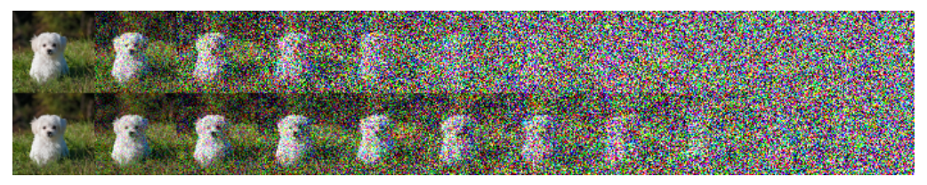
The forward diffusion process is an essential component of Diffusion Models, where a clean data sample is progressively transformed into a noisier version over multiple steps.
Given a data sample \(x_0\) with a distribution \(x_0 \sim q(x_0)\), the forward diffusion process generates a sequence of increasingly noisy versions of this data by adding Gaussian noise at each of \(T\) steps. The noise introduced at each step \(t\) is characterized by a variance parameter \(\beta_t \in [0, 1]\). The conditional distribution of \(x_t\) given \(x_{t-1}\) is defined as:
\[q(x_t \mid x_{t-1}) = \mathcal{N}\left(x_t; \sqrt{1-\beta_t} \cdot x_{t-1}, \beta_t \mathbf{I}\right)\]Here, \(q(x_t \mid x_{t-1})\) represents a Gaussian distribution where \(x_t\) has a mean of \(\sqrt{1-\beta_t} \cdot x_{t-1}\) and a variance of \(\beta_t \mathbf{I}\). As \(t\) increases, \(x_0\) gradually loses its original features. In the limit as \(t \to \infty\), \(x_T\) becomes an isotropic Gaussian distribution:
\[x_T \sim \mathcal{N}(0, \mathbf{I})\]The distribution of the final noisy sample \(x_T\) given the initial data \(x_0\) can be expressed as:
\[q(x_{1:T} \mid x_0) = \prod_{t=1}^{T} q(x_t \mid x_{t-1})\]This equation describes a Markov chain, where the distribution of \(x_t\) depends solely on the previous state \(x_{t-1}\). To simplify the notation, we define \(\alpha_t = 1 - \beta_t\) and \(\bar{\alpha}t = \prod{i=1}^{t} \alpha_i\). Using these definitions, we can express \(x_t\) as:
\[x_t = \sqrt{\alpha_t} x_{t-1} + \sqrt{1-\alpha_t} \epsilon_{t-1}\] \[= \sqrt{\alpha_t \alpha_{t-1}} x_{t-2} + \sqrt{1-\alpha_t \alpha_{t-1}} \bar{\epsilon}_{t-2}\] \[\vdots\] \[= \sqrt{\bar{\alpha}_t} x_0 + \sqrt{1-\bar{\alpha}_t} \epsilon\]Thus, the distribution of \(x_t\) given \(x_0\) can be rewritten as:
\[q(x_t \mid x_0) = \mathcal{N}\left(x_t; \sqrt{\bar{\alpha}_t} \cdot x_0, (1 - \bar{\alpha}_t) \mathbf{I}\right)\]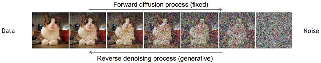
Inverse Diffusion
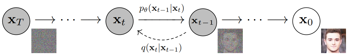
The inverse diffusion process is the core generative mechanism in Diffusion Models. If we can reverse the process \(q(x_{t-1} \mid x_t)\), we will be able to re-create the true input data \(x_0\), knowing that \(q(x_{t-1} \mid x_t)\) is also a Gaussian.
Unfortunately, the estimation of \(q(x_{t-1} \mid x_t)\) is intractable, so we need to approximate the process by using a learned model \(p_{\theta}\) to estimate the reverse process, where:
\[p_{\theta}(x_{t-1} \mid x_t) = \mathcal{N}\left(x_{t-1}; \mu_{\theta}(x_t, t), \sigma_{\theta}(x_t, t)\right)\]The parameters \(\mu_{\theta}(x_t, t)\) and \(\sigma_{\theta}(x_t, t)\) are learned by the model, and they represent the mean and standard deviation of the Gaussian distribution at each step \(t\).
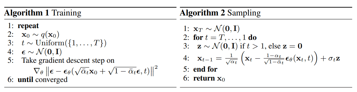
Training Diffusion Models
Training Diffusion Models involves optimizing the parameters of the model. Specifically, we aim to train \(\mu_{\theta}\) to predict the mean \(\mu_t\) of the reverse process, given by:
\[\mu_{t} = \frac{1}{\sqrt{\alpha_{t}}}\left(x_{t} - \frac{1-\alpha_{t}}{\sqrt{1-\bar{\alpha}_{t}}} \epsilon_{t}\right)\]After a sequence of simplifications, which will be detailed in the next section, the loss function can be expressed as:
\[L_{t} = \mathbb{E}_{x_{0},t,\epsilon} \left[ \frac{1}{2 ||\sigma_{\theta}(x_{t},t)||_{2}^{2}} ||\mu_{t} - \mu_{\theta}(x_{t},t)||_{2}^{2}\right]\] \[= \mathbb{E}_{x_{0},t,\epsilon} \left[ \frac{\beta_{t}^{2}}{2 \alpha_{t} (1-\bar{\alpha}_{t}) ||\sigma_{\theta}||_{2}^{2}} ||\epsilon_{t}-\epsilon_{\theta}(\sqrt{\bar{\alpha}_{t}}x_{0} + \sqrt{1-\bar{\alpha}_{t}}\epsilon_{t})||^{2} \right]\]Thus, instead of directly predicting the mean of the Gaussian distribution, we predict the noise \(\epsilon_t\) that is added to the input \(x_0\) to generate the output \(x_t\) at each step \(t\).
Parametrisation
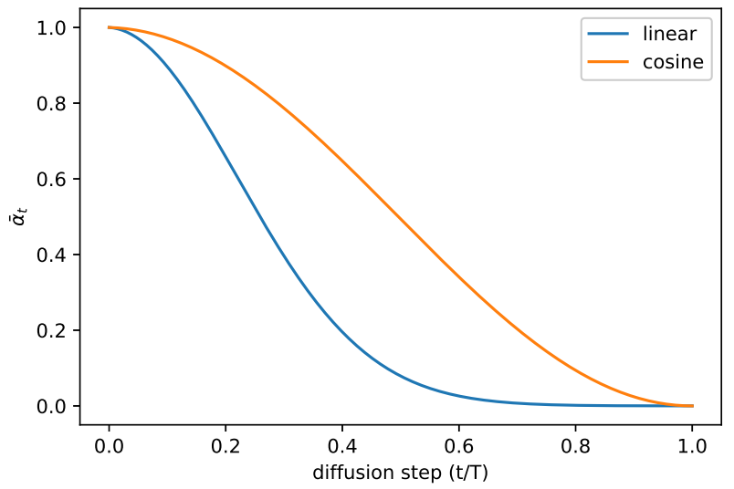
The forward variance \(\beta_{t}\) can be set as a constant or determined by a schedule over time \(T\).
Linear: In this approach, the variance increases linearly with \(t\), forming a sequence of constants \(\beta_{1}, \beta_{2}, \ldots, \beta_{T}\), where \(\beta_{1} < \beta_{2} < \ldots < \beta_{T}\). These values should be chosen relatively small compared to the normalized input \(x_{0} \in [-1, 1]\). Common choices include \(\beta_{1} = 10^{-4}\) and \(\beta_{T} = 0.02\).
Cosine: An improvement over the linear schedule is the use of a cosine-based variance schedule, which is defined by the following equations:
\[ \bar{\alpha}{t} = \frac{f(t)}{f(0)}, \quad f(t) = \cos^2{\left(\frac{t/T + s}{1 + s} \cdot \frac{\pi}{2}\right)}, \quad \beta{t} = \text{clip}\left(1 - \frac{\bar{\alpha}{t}}{\bar{\alpha}{t-1}}, 0.999\right) \]
Model Architectures
Diffusion Models can be implemented using various neural network architectures, each with its unique strengths and applications. The common architectures include U-Net and transformers.
U-Net Architecture
The U-Net architecture is commonly used due to its ability to handle inputs and outputs of the same spatial size. The U-Net consists of:
Downsampling: This part reduces the spatial dimensions of the input while increasing the number of feature channels. It involves repeated 3x3 convolutions followed by ReLU activations and 2x2 max pooling with stride 2.
Upsampling: This component reconstructs the original spatial dimensions from the compressed representation. It includes upsampling of the feature maps followed by 2x2 convolutions.
Skips: These connections link corresponding layers from the downsampling and upsampling branch. They concatenate features from the encoder with the decoder, preserving high-resolution details.
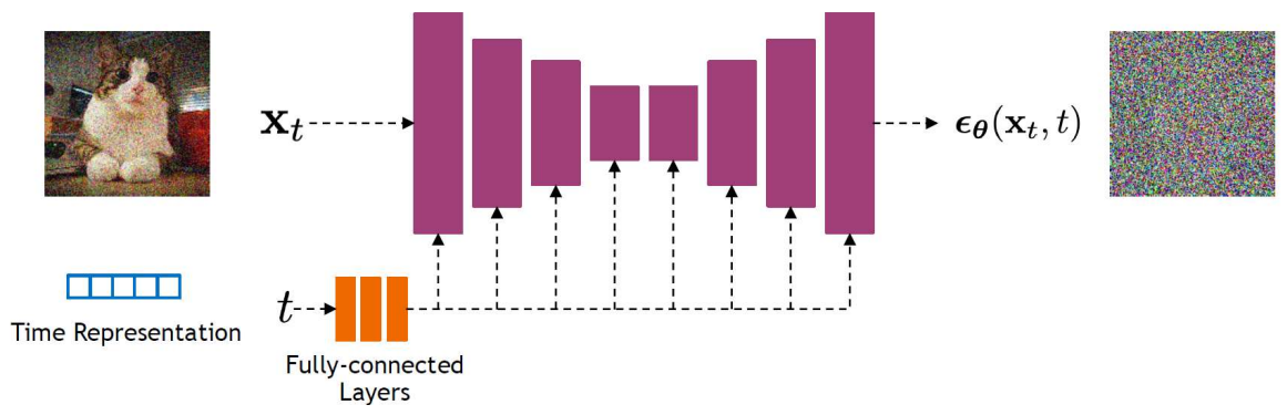
The original implementation of the U-Net in diffusion models uses ResNet blocks with diffusion time step embeddings, Swish non-linearity, and group normalization. Additionally, an attention block was introduced.
Transformer-Based Models
Conditional Generation
Diffusion Models can be extended to perform conditional generation, which allows for the generation of data based on additional information such as text descriptions or class labels. This approach enhances the model’s capability to produce outputs that are aligned with specific conditions, providing greater control over the generated data.
In conditional generation, an additional input, such as a text description or class label, is integrated into the diffusion process. This conditioning guides the generation of images or other types of data to match the specified condition. Mathematically, the conditional distribution of \(x_t\) given \(x_{t-1}\) and the condition \(y\) is expressed as:
\[p_{\theta}(x_{0:T} \mid y) = p(x_{T})\prod_{t=1}^{T} p_{\theta}(x_{t-1} \mid x_{t}, y)\]where the conditional probability \(p_{\theta}(x_{t-1} \mid x_{t}, y)\) follows a Gaussian distribution with mean \(\mu_{\theta}(x_t, t, y)\) and variance \(\sigma_{\theta}(x_t, t, y)\):
\[p_{\theta}(x_{t-1} \mid x_{t}, y) = \mathcal{N}\left(x_{t-1}; \mu_{\theta}(x_t, t, y), \sigma_{\theta}(x_t, t, y)\right)\]Classifier-Guided Diffusion
A common technique in conditional generation is classifier-guided diffusion. This involves training a classifier \(f_{\phi}(y \mid x_{t}, t)\) to provide guidance based on the noisy image \(x_t\) and the condition \(y\). The classifier helps steer the diffusion process towards generating data that aligns with the given condition by leveraging gradients.
The gradient of the log probability of the classifier is used to influence the diffusion process. Specifically, the gradient of the log of a Gaussian distribution is given by:
\[\nabla_{x} \log \mathcal{N}(x; \mu, \sigma) = \frac{x - \mu}{\sigma^2} = \frac{\epsilon}{\sigma}\]where \(\epsilon \sim \mathcal{N}(0, I)\). This relates to the noise added during the diffusion process.
The gradient of the diffusion process with respect to the noisy image \(x_t\) is:
\[\nabla_{x_{t}} \log q(x_{t}) = - \frac{\epsilon_{\theta}(x_{t}, t)}{\sqrt{1-\bar{\alpha}_{t}}}\]where \(\epsilon_{\theta}(x_{t}, t)\) represents the predicted noise at time \(t\).
To incorporate the classifier’s guidance, the joint distribution gradient is expressed as:
\[\nabla_{x_{t}} \log q(x_{t}, y) = \nabla_{x_{t}} \log q(x_{t}) + \nabla_{x_{t}} \log q(y \mid x_{t})\] \[\approx - \frac{\epsilon_{\theta}(x_{t}, t)}{\sqrt{1-\bar{\alpha}_{t}}} + \nabla_{x_{t}} \log f_{\phi} (y \mid x_{t})\] \[= - \frac{1}{\sqrt{1-\bar{\alpha}_{t}}}(\epsilon_{\theta}(x_{t}, t)) - \sqrt{1-\bar{\alpha}_{t}} \nabla_{x_{t}} \log f_{\phi} (y \mid x_{t}, t)\]This formulation results in a new classifier-guided noise predictor \(\bar{\epsilon}_{\theta}\):
\[\bar{\epsilon}_{\theta}(x_{t}, t) = \epsilon_{\theta}(x_{t}, t) - \sqrt{1-\bar{\alpha}_{t}} \nabla_{x_{t}} \log f_{\phi} (y \mid x_{t}, t)\]To further control the influence of the classifier, a scaling factor \(s\) is introduced:
\[\bar{\epsilon}_{\theta}(x_{t}, t) = \epsilon_{\theta}(x_{t}, t) - \sqrt{1-\bar{\alpha}_{t}} s \nabla_{x_{t}} \log f_{\phi} (y \mid x_{t}, t)\]This scaling allows for adjusting the strength of the classifier’s guidance during the diffusion process, providing flexibility in balancing between the model’s inherent noise prediction and the external condition.
This version aims to provide clearer explanations and context for each part of the conditional generation process and the role of classifier-guided diffusion in improving control over the generated outputs.
Classifier-Free Guided Diffusion
Classifier-Free Guided Diffusion eliminates the need for a separate classifier by using a single network to handle both conditional and unconditional diffusion models. This approach allows for guidance without explicitly training an additional classifier.
In this framework, \(p_{\theta}(x)\) represents the unconditional diffusion model, with a score estimator \(\epsilon_{\theta}(x, t)\), while \(p_{\theta}(x \mid y)\) denotes the conditional diffusion model, with a score estimator \(\epsilon_{\theta}(x, t, y)\). The unconditional model is a special case of the conditional model when no condition \(y\) is provided.
The gradient of the implicit classifier can be expressed using both conditional and unconditional score estimators:
\[\nabla_{x_{t}} \log p(y \mid x_{t}) = \nabla_{x_{t}} \log p(x_{t} \mid y) - \nabla_{x_{t}} \log p(x_{t})\]Approximating this, we get:
\[\nabla_{x_{t}} \log p(y \mid x_{t}) \approx - \frac{1}{\sqrt{1-\bar{\alpha}_{t}}} \epsilon_{\theta}(x_{t}, t, y) - \epsilon_{\theta}(x_{t}, t)\]The guided noise predictor, which incorporates this implicit classifier gradient, is defined as:
\[\bar{\epsilon}_{\theta}(x_{t}, t, y) = \epsilon_{\theta}(x_{t}, t, y) - \sqrt{1-\bar{\alpha}_{t}} s \nabla_{x_{t}} \log p(y \mid x_{t})\]Substituting the gradient expression, this becomes:
\[\bar{\epsilon}_{\theta}(x_{t}, t, y) = \epsilon_{\theta}(x_{t}, t, y) + s (\epsilon_{\theta}(x_{t}, t, y) - \epsilon_{\theta}(x_{t}, t))\]or simplified to:
\[\bar{\epsilon}_{\theta}(x_{t}, t, y) = (1 + s) \epsilon_{\theta}(x_{t}, t, y) - s \epsilon_{\theta}(x_{t}, t)\]Cascaded Diffusion Models
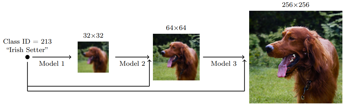
Cascaded Diffusion Models were proposed to generate high-resolution images. To generate an image, we sample a low-resolution image from the first model and then use it as input to the second model to generate a higher-resolution image. This process can be repeated multiple times to generate images of even higher resolutions.
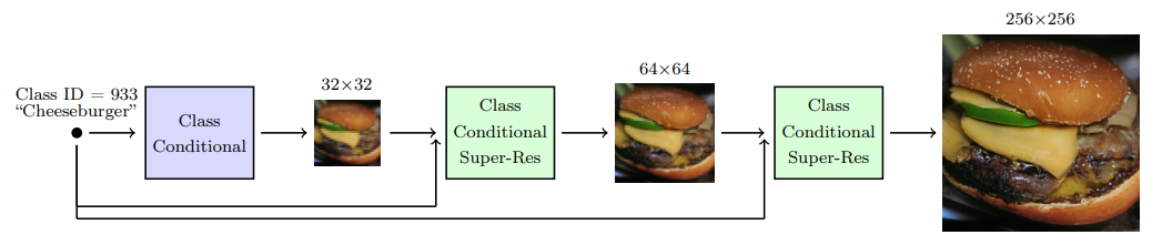
Noise Conditioning Augmentation: Diffusion models are trained on low-resolution datasets, with noisy generated images and artifacts. To improve the quality of the generated images, noise conditioning augmentation is used. The technique involves adding noise to the input image during training (e.g., Gaussian blur) to make the model more robust to noise and improve the quality of the generated images.
Latent Diffusion Models
Latent Diffusion Models (LDM), or Stable Diffusion Models, are a variant of diffusion models that use the latent representation in the diffusion process instead of the pixel/image representation. Compared to the high-dimensional pixel space, the latent space focuses on the important semantics/features of the input image, reducing training time and inference speed.
The autoencoder \(G\) is used to encode the image \(x \in \mathbb{R}^{CHW}\) into a latent representation \(z \in \mathbb{R}^{d}\), where \(z = G(x)\). Then, the decoder \(D\) is used to reconstruct the image \(x’\) from the latent representation \(z\) as \(x’ = D(z)\).
Thus the objective of the LDM can be formulated as:
\[L = E_{G(x), \epsilon \sim \mathcal{N}(0,1), t} \left[ \| \epsilon - \epsilon_{\theta}(z_{t}, t) \|_{2}^2 \right]\]The Conditioning Mechanism: The latent diffusion model can be conditioned on \(y\), a text description, to generate images that align with it. The conditioning is introduced at the level of the U-Net, where a cross-attention mechanism is used to fuse the projected condition \(y\) with the latent representation \(z\) using a domain-specific encoder \(\tau_{\theta} \in \mathbb{R}^{M \times d_r}\).
\[\text{Attention}(Q, K, V) = \text{softmax}\left(\frac{QK^T}{\sqrt{d_k}}\right)V\]Where:
- \(Q = W_q \cdot \phi(z)\)
- \(K = W_k \cdot \tau_{\theta}(y)\)
- \(V = W_v \cdot \tau_{\theta}(y)\)
With:
- \(\phi(z) \in \mathbb{R}^{N \times d_{\epsilon}}\)
- \(\tau_{\theta}(y) \in \mathbb{R}^{M \times d_r}\)
- \(W_q \in \mathbb{R}^{d \times d_{\epsilon}}\),
- \(W_k \in \mathbb{R}^{d \times d_r}\),
- \(W_v \in \mathbb{R}^{d \times d_r}\)
Based on image conditioning, the LDM is learned via:
\[L = E_{G(x), \epsilon \sim \mathcal{N}(0,1), t} \left[ \| \epsilon - \epsilon_{\theta}(z_{t}, t, y) \|_{2}^2 \right]\]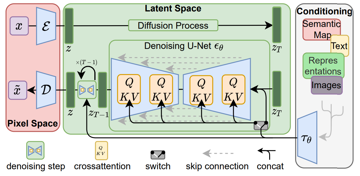
Regularization: The latent diffusion model can be regularized to prevent high variance in the latent space.
- KL-reg: a slight KL penalty on the latent space toward standard normal.
- VQ-reg: uses a vector quantization layer within the decoder.