State Space Models (SSM)
Published:
Welcome to this guide on State Space Models (SSMs), exploring their efficiency in modeling long-range dependencies, the S4 model, and key techniques.
Table of Contents
Introduction
State Space Models (SSMs)
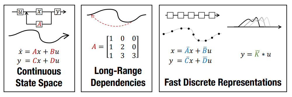
Sequence modeling is central to many machine learning tasks. A persistent challenge is modeling long-range dependencies (LRDs). Recurrent Neural Networks (RNNs), Convolutional Neural Networks (CNNs), and Transformers have specialized variants designed to capture these dependencies, yet they often struggle to scale efficiently with very long sequences.
State space models (SSMs) have emerged as a promising alternative for sequence modeling, providing a principled way to represent system states and their transitions over time. The Structured State Space (S4) model, introduced by Gu et al. (2021), overcomes prior limitations of SSMs by efficiently capturing long-range dependencies while minimizing computational and memory bottlenecks.
SSMs vs. Transformers
Transformers are popular in sequence modeling because their self-attention mechanisms can capture long-range dependencies. However, the quadratic complexity of self-attention limits their scalability for very long sequences. In contrast, SSMs provide a more efficient way to model long-range dependencies by combining continuous-time, recurrent, and convolutional properties.
The Future of SSMs
The S4 model is a significant advancement in sequence modeling, offering a robust alternative to existing techniques for tasks requiring efficient handling of long-range dependencies. It provides a strong foundation for future developments in sequence modeling.
In this post, we’ll explore the key concepts behind the Structured State Space (S4) model and its applications in sequence modeling.
Structured State Space (S4)
State Space Models (SSMs)
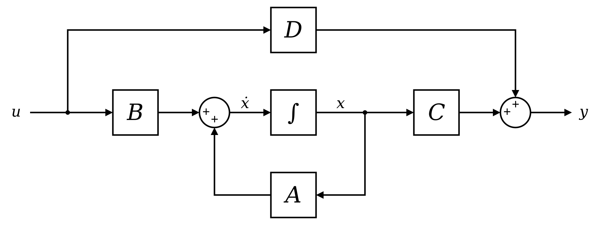 Figure 1: Block diagram representation of the linear state-space equations.
State space models (SSMs) are a class of probabilistic models that describe a system’s evolution over time. They consist of two primary components:
State Equation: Models the system’s internal dynamics
\(\dot{x}(t) = f(x(t), u(t))\)Observation Equation: Relates the system’s internal state to observed data
\(y(t) = g(x(t), u(t))\)
We note that SSMs are widely used in control theory and signal processing to model complex systems with hidden states, such as Kalman filters and Hidden Markov Models (HMMs).
The SSM model is defined by learned parameters \({A, B, C}\), where:
- \(A\): State transition matrix
- \(B\): Input matrix
- \(C\): Observation matrix
- \(D\): Feedforward matrix (typically set to zero, i.e., \(D = 0\))
The system equations are:
\[\begin{aligned} \dot{x}(t) &= A x(t) + B u(t) \\ y(t) &= C x(t) \end{aligned}\]We can say that the SSM maps a 1D input signal \(u(t)\) to a latent state \(x(t) \in \mathbb{R}^{p \times D}\), which is then mapped to an output signal \(y(t) \in \mathbb{R}^{q \times D}\).
HiPPO: High-order Polynomial Projection Operators
State space models have an exponential nature, which causes SSMs to suffer from gradient explosion or vanishing when handling long sequences—making them impractical for capturing long-range dependencies.
To address this, the authors introduced HiPPO theory, which allows the state \(x(t)\) to memorize the input \(u(t)\) through a state transition matrix \(A\), called the HiPPO matrix. At any time \(t\), the state \(x(t)\) can approximately reconstruct the entire past input up to \(t\).
The HiPPO matrix is defined as:
\[A_{n,k} = - \left\{ \begin{array}{ll} \sqrt{2n + 1} \sqrt{2k + 1} & \text{if } n > k \\\\ n + 1 & \text{if } n = k \\\\ 0 & \text{if } n < k \end{array} \right.\]🧠 For the MNIST benchmark, introducing this matrix improved performance from 60% to 98% accuracy 🎉
Discrete-Time SSMs
To model sequence-to-sequence tasks using SSMs, we discretize the continuous-time formulation by introducing a step size \(\Delta\), leading to:
\[\begin{aligned} x_k &= \bar{A} x_{k-1} + \bar{B} u_k \\\\ y_k &= \bar{C} x_k \end{aligned}\]Using the bilinear transformation, we approximate the derivative as:
\[\frac{x(t + \Delta) - x(t)}{\Delta} \approx \frac{1}{2} \left[ A x(t + \Delta) + B u(t + \Delta) + A x(t) + B u(t) \right]\]Rearranging:
\[x(t + \Delta) - x(t) = \frac{\Delta}{2} \left[ A x(t + \Delta) + B u(t + \Delta) + A x(t) + B u(t) \right]\]Solving for \(x(t + \Delta)\):
\[x_{k+1} = \left(I - \frac{\Delta}{2} A\right)^{-1} \left( \left(I + \frac{\Delta}{2} A\right) x_k + \frac{\Delta}{2} \left(B u_{k+1} + B u_k\right) \right)\]Letting:
\[\begin{aligned} \bar{A} &= \left(I - \frac{\Delta}{2} A\right)^{-1} \left(I + \frac{\Delta}{2} A\right) \\\\ \bar{B} &= \left(I - \frac{\Delta}{2} A\right)^{-1} \Delta B \\\\ \bar{C} &= C \end{aligned}\]We obtain a discrete-time SSM suitable for sequence modeling tasks, where the observation equation remains unchanged.
Training SSMs: the Convolutional Representation
For non-recurrent SSMs, we can draw a connection between Linear Time-Invariant (LTI) systems and convolutional neural networks. Assuming the initial state \(x_0 = 0\), the output of the SSM can be written step-by-step:
\[\begin{array}{ccc} k = 0 \left\{ \begin{aligned} x_0 &= \bar{B} u_0 \\ y_0 &= \bar{C} x_0 = \bar{C} \bar{B} u_0 \end{aligned} \right. & k = 1 \left\{ \begin{aligned} x_1 &= \bar{A} x_0 + \bar{B} u_1 = \bar{A} \bar{B} u_0 + \bar{B} u_1 \\ y_1 &= \bar{C} x_1 = \bar{C} \bar{A} \bar{B} u_0 + \bar{C} \bar{B} u_1 \end{aligned} \right. & k = 2 \left\{ \begin{aligned} x_2 &= \bar{A} x_1 + \bar{B} u_2 = \bar{A}^2 \bar{B} u_0 + \bar{A} \bar{B} u_1 + \bar{B} u_2 \\ y_2 &= \bar{C} x_2 = \bar{C} \bar{A}^2 \bar{B} u_0 + \bar{C} \bar{A} \bar{B} u_1 + \bar{C} \bar{B} u_2 \end{aligned} \right. \end{array}\]The output sequence \(y_k\) can be vectorized as a convolution:
\[\begin{aligned} y_k &= \sum_{i=0}^{k} \bar{C} \bar{A}^{k-i} \bar{B} u_i \\ &= \bar{C} \bar{A}^k \bar{B} u_0 + \bar{C} \bar{A}^{k-1} \bar{B} u_1 + \dots + \bar{C} \bar{B} u_k \\ &= \bar{K} * u \end{aligned}\]Where \(\bar{K}\), the SSM convolutional kernel, is given by:
\[\bar{K} = \begin{bmatrix} \bar{C} \bar{A}^k \bar{B} \\ \bar{C} \bar{A}^{k-1} \bar{B} \\ \vdots \\ \bar{C} \bar{A} \bar{B} \\ \bar{C} \bar{B} \end{bmatrix}\]This formulation allows SSMs to be trained like 1D convolutional models, making them efficient for sequence modeling.
Methods
Diagonalization of the HiPPO Matrix
We have shown that the discrete SSM involves repeated multiplication of the matrix \(\bar{A}\), which requires:
- Time complexity: \(O(N^2 L)\)
- Memory complexity: \(O(N L)\)
where \(N\) is the number of states and \(L\) is the sequence length.
Assuming \(x = V \hat{x}\), we can diagonalize the state-space model as:
\[\begin{aligned} \dot{\hat{x}} &= V^{-1} A V \hat{x} + V^{-1} B u \\\\ y &= C V \hat{x} \end{aligned}\]For a diagonal matrix \(A\), the system can be solved in:
\[O(NL \log^2(N + L))\]This is possible because \(\bar{K}\) becomes a Vandermonde matrix, allowing fast computation. However, in practice, diagonalizing the HiPPO matrix is numerically unstable.
Normal Plus Low-Rank (NPLR) Decomposition
Although the HiPPO matrix is not diagonalizable directly due to its structure, it can be decomposed into a normal matrix and a low-rank matrix:
\[\text{HiPPO} = \text{Normal} + \text{Low-Rank}\]- The Normal component is diagonalizable
- The Low-Rank component enables expressivity
This structure enables more efficient computation while preserving modeling capacity.
Using this decomposition, the complexity is also reduced to:
\[O(NL \log^2(N + L))\]Despite the fact that summing diagonal and low-rank parts is slower than purely diagonal systems, the authors proposed algorithmic improvements to overcome these limitations.
References
[1] Efficiently Modeling Long Sequences with Structured State Spaces, Albert Gu, Karan Goel, and Christopher Ré.