Coordinate-based Networks

Table of Contents

1. Introduction
2. Definition
3. Representations - Voxel - Point - Mesh - Occupancy Networks
   • Appearance, Geometry, and Surfaces properties
   • Convolutional Occupancy Networks
4. Mesh Extraction - Marching Cubes - Multiresolution Iso-Surface Extraction (MISE)
5. Differentiable Volumetric Rendering
6. Neural Radiance Fields
7. References

Introduction

In this tutorial, we will approach the Neural Implicit Representation principals and its applications in computer vision, graphics, and robotics.

Definition

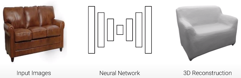
Implicit Neural Representation (INR) is a novel concept within machine learning and computer graphics that represents an object or scene as a continuous function, rather than an explicit surface or structure. Implicit Neural Representation aims to learn a mathematical function $ f(x, y) = 0 $ or implicit representation that can generate the desired data points.

Learning-based approaches for 3D reconstruction have gained popularity for its rich representation to 3D models, compared to the traditional Multi View Stereo (MVS) algorithms. Through literature, Deep learning approaches are categorized into three representations:

Representations

What is a good representation ?

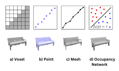
Voxel

Voxel are easy to process by neural network and commonly used in generative 3D tasks, by discretizing the space into a set of 3D voxel grids. However, Due to its cubic memory $O(n^3)$, the voxels representations are limited to small resolutions of the underlying 3D grid. [2]

Point

As an alternative to the voxel representation, the output can be represented as a set of 3D point clouds.However, the point representation doesn’t preserve the model connectivity and topology, hence require a post-processing steps to extract 3D mesh. The point representation is also limited by the number of points, which affects the resolution of the final model. [3]

Mesh

Representing the output as a set of triangles (vertices and faces) is a very complicated structure that requires reference template from the same object class. Yet, the approach is still limited by the memory requirements and the resolution of the mesh. [4]

Occupancy Networks

the Occupancy Networks implicitly represents the 3D surface as a decision boundary of a nonlinear classifier, and for every point $\mathbf{p} \in \mathbb{R}^3$ in the 3D space, the network predicts the probability of the point being inside the object. The occupancy function is defined as:

The occupancy function is approximated by a deep neural network $f_\theta$ with parameters $\theta$ that takes an observation $\mathbf{x} \in X$ as input condition (ex. image, point clouds,…), and it has a function from $\mathbf{p} \in \mathbb{R}^3$ to $\mathbb{R}$ as an occupancy probability.

For each input pair $(p,x)$, we can write the occupancy network function as:

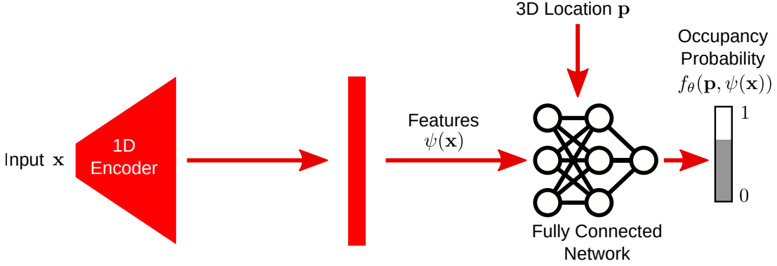
The advantage of the occupancy network is a continuous representation with an infinite resolution, the representation is not restricted to a specific class as in the mesh representation and it has a low memory footprint.

To learn the parameters $\theta$, we randomly sample 3D points (ex. $K=2048$) in the volume and minimize the binary cross-entropy $BCE$ loss function:

• In practice, we sample the 3D points uniformly inside the bounding box of the object.

Appearance, Geometry, and Surfaces properties

The implicit representation can be extended to have more objects properties and reasoning, such as the surface lightening and the view point. The occupancy network can conditioned by the viewing direction $v$ and light location $l$ for any 3D point $p$, for each input tuple $(p,v,l)$, we can write the occupancy network function as:

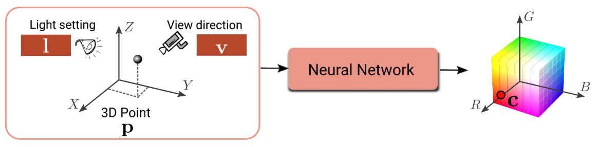
The network encodes both an input 2D image and the corresponding 3D shape into a latent representations $z$ and $s$, as a conditioning to the occupancy network. The model predicts the occupancy probability for each 3D point $p$ and the color $c$, Surface Light Fields.

• The light $l$, denotes the light source parameters, such as the light direction, color, and intensity.

The network is trained to minimize the photometric loss function between the predicted image $I$ and the input image $\hat{I}$:

Convolutional Occupancy Networks

Large-scale representation learning for 3D scenes ?

Implicit Neural Representations have demonstrates a good results for small objects and small scenes, however, most of approaches fails to scale to large scenes, due to:

• The previous architectures does incorporate the local information in the observation.
• It doesn’t exploit and capture the translational equivariance of the 3D scene.

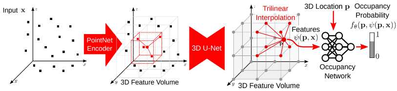
The Convolutional Occupancy Networks introduces the convolutional networks into the implicit modeling for an accurate and rich large scale 3D scenes. The convolutional network incorporates the local as well the global information, and the inductive biases to obtain a better generalization, more specifically the translation equivariance.

We process the inputs thought an encoder to extract feature embeddings, we use PointNet for input point clouds and a 3D-CNN for a input voxel.

• Planar Encoding:

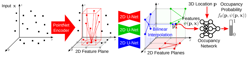
For each input point, we perform an orthographic projection onto a canonical plane, aligned with the axes of the coordinate frame, which we discretize at a resolution of H × W pixel cells.

We aggregate features projecting onto the same pixel using average pooling, resulting in planar features with dimensionality $H × W × d$.

• Volume Encoding:

The volumetric encodings represents the 3D information better than a 2D planar, However, the resolution is restricted by the memory footprint. The average pooling is performed all over the voxel cell, resulting in a feature volume with dimensionality $H × W × D × d$.

• Convolutional Decoder:

The convolutional decoder processes the resulting feature planes and feature volumes using 2D and 3D U-Net network to aggregate the local and global information, and the equivariance to translation properties in the output features, enabling structured reasoning.

• Occupancy Prediction:

Given the aggregated features, we predict the occupancy probability for each 3D point $p$ by projecting each point onto the corresponding plane and query the feature vector using bilinear interpolation. For multiple planes, we sum the features of all planes. For the volume, we query the feature vector using trilinear interpolation.

For a resulting feature vector $x$ at point $p$, denoted as $\psi(p,x)$, we predict the occupancy probability using fully connected layers occupancy network, as:

• In comparison to the occupancy network, the convolutional occupancy network has a better accuracy and a faster convergence.

• The convolutional occupancy network shows a good generalization and scalability for large scenes, we can use a hierarchical approach to process the scene using sliding window.

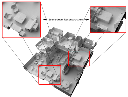
Mesh Extraction

The mesh extraction is a post-processing step that extracts the 3D mesh from the occupancy network.

Marching Cubes

The marching cubes algorithm is a method for extracting a polygonal mesh of an isosurface from a 3D scalar field. The iso-surface is formed by connecting the vertices of the cubes that are intersected by the iso-surface.

Algorithm:

• We divide the 3D space into a grid of cubes (8 vertices).
• For each cube, we evaluate the cube vertices and compare them to the threshold value $\tau$.
• We construct a triangulation for each cube, based on the vertices that are intersected by the iso-surface.
• Based on the triangulations, We generate polygons for each cube and we merge the polygons to form the final mesh.
• We optimize the mesh by removing the duplicated vertices and edges.

Multiresolution Iso-Surface Extraction (MISE)

MISE is a method that incrementally building an octree to extract high resolution meshes from the occupancy function.

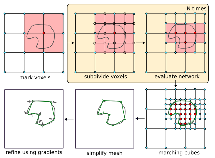
• We divide the 3D space into an initial resolution (ex. $32^2$), and we compute the occupancy function $f_\theta(p,x)$ for each cell.

• We set a threshold value $\tau$ and we mark a grid points “occupied” if the occupancy function $f_\theta(p,x)$ is greater than the threshold.

• We subdivide the query space into 8 sub-cells and we evaluate the occupancy function $f_\theta(p,x)$ for each cell.

• We repeat the process until we reach the desired resolution.

• At the end, we apply the marching cubes algorithm to extract an approximate iso-surface, defined by the threshold value $\tau$: { $ \ p \in \mathbb{R}^3 \ \

  \ \ f_\theta(p, x) = \tau $ }

Differentiable Volumetric Rendering

Learning from images only !

Learning based 3D reconstruction methods have shown impressive results, however these methods require 3D supervision from the real world or synthetic data.

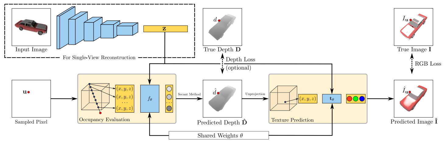
Differentiable Rendering aims to learn 3D reconstruction from RGB images only, by using the concept of implicit representation in deriving the depth gradients.

The input image is processed with an encoder to extract latent representation $z \in \mathbb{Z} $ as a conditioning to the occupancy network $f_\theta$, as introduced in the Occupancy Networks. The 3D surface shape is determined by a threshold value $\tau$, such as $f_\theta(p, z) = \tau$.

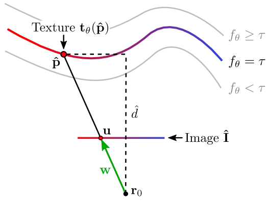
The texture of a 3D shape can be described using a texture field $t_\theta: \mathbb{R}^3 \times \mathbb{Z} \rightarrow \mathbb{R}^3$; which regresses the RGB color value for every point $p \in \mathbb{R}^3 $, conditioned on the same latent representation $z \in \mathbb{Z}$. The texture of an object is determined by the value of $t_\theta$ at the surface $f_\theta = \tau$.

We define the photometric loss function between the input image $I$, and the rendered image $\hat{I}$ as:

• $u$ denotes the pixel location in the image.

For a camera located at $r_0$, we can render the image $\hat{I}$ at pixel location $u$ by casting a ray from the camera center $r_0$ through the pixel location $u$, and we compute the intersection point $\hat{p}$ with the surface $f_\theta(p) = \tau$.

For any pixel $u$, this ray can written as $\hat{p} = r_0 + d \cdot w$, where $d$ is the depth value. Since $\hat{p}$ depends on $\theta$. The partial derivative of $\hat{p}$ with respect to $\theta$ can be computed using the chain rule:

Applying the chain rule to the photometric loss function $L$ , we can compute the partial derivative of the loss function with respect to $\theta$ as:

Solving for $\frac{\partial \hat{p}}{\partial \theta}$, we can write the partial derivative of the loss function with respect to $\theta$ as:

Calculating the gradient of the surface depth $\hat{d}$ with reference to the network parameters $\theta$ only involves calculating the gradient of $f_{\theta}$ at $\hat{p}$ with reference to the network parameters $\theta$ and the surface point $\hat{p}$.

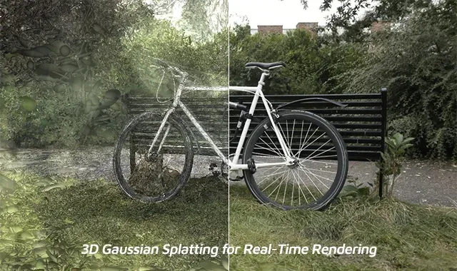
Neural Radiance Fields

Can we render a novel photo-realistic view of the scene from an implicit representation ?

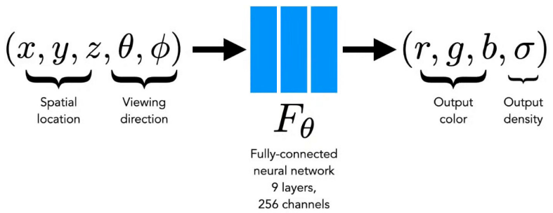
Neural Radiance Fields (NeRF) is a method for synthesizing novel views of a scene from a sparse set of input views. NeRF maps a 3D spatial location $\mathbf{x} \in \mathbb{R}^3$ and a 2D viewing direction $\mathbf{d} \in \mathbb{R}^2$ to color $\mathbf{c} \in \mathbb{R}^3$ and density $\sigma \in \mathbb{R}$, The network function is represented as a MLP network and defined as:

• Density $\sigma$ describes the opacity of a 3D point in the scene. For a consistent multi-view representation, we predict the density $\sigma$ from the input location $\mathbf{x}$ only.

• The color $\mathbf{c}$ is predicted from the input location $\mathbf{x}$ and the viewing direction $\mathbf{d}$.

• $d$ represents the viewing direction, which is the direction from the camera center to the 3D point.

Unlike to DVR, NeRF doesn’t evaluate the color on the ray at the surface, instead it evaluates the color/density at multiple points along the ray by integrating the color/density along the ray.

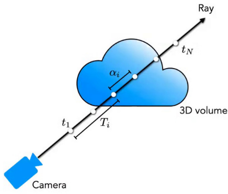
The rendering equation for a ray $r(t) = r_0 + t \cdot d$ is defined as:

• $ci$ is the color of the $i$-th point along the ray, and $T_i$ is the weight.

• Alpha $\alpha_{i}$ is the accumulated density along the ray, and it is defined as:

\(\alpha_{i} = 1 - \exp^{(-\sigma_{i} \cdot \Delta t)}\) NeRF Model:

class NeRF(nn.Module):
    def __init__(self, in_features=3, hidden_features=256, out_features=4, num_layers=8, viewdir_features=128):
        super(NeRF, self).__init__()

        # Define MLP for volume density prediction
        self.density_mlp = self._make_mlp(in_features, hidden_features, out_features, num_layers)

        # Define MLP for view-dependent RGB color prediction
        self.viewdir_mlp = self._make_mlp(in_features + viewdir_features, hidden_features, out_features, 1)

    def _make_mlp(self, in_features, hidden_features, out_features, num_layers):
        layers = []
        for _ in range(num_layers):
            layers.append(nn.Linear(in_features, hidden_features))
            layers.append(nn.ReLU())
            in_features = hidden_features
        layers.append(nn.Linear(hidden_features, out_features))
        return nn.Sequential(*layers)

    def forward(self, coords, view_dir):
        # Process input coordinates with density MLP
        density_feature = self.density_mlp(coords)
        sigma = torch.sigmoid(density_feature[:, 0])  # Extract sigma from the output

        # Concatenate the feature vector with view direction
        view_input = torch.cat([density_feature[:, 1:], view_dir], dim=1)

        # Predict view-dependent RGB color using viewdir MLP
        color = torch.sigmoid(self.viewdir_mlp(view_input))

        return sigma, color

NeRF Training: We sample a set of rays from the input images, and we optimize the network parameters $\theta$ to minimize the reconstruction loss function:

# loss
def nerf_loss(sigma, color, target_color):
    # Compute the accumulated density along the ray
    alpha = 1 - torch.exp(-sigma * delta_t)

    # Compute the predicted color along the ray
    pred_color = torch.exp(-alpha * sigma) * color

    # Compute the reconstruction loss
    loss = torch.mean(torch.sum((pred_color - target_color) ** 2, dim=-1))
    return loss

• The sampling strategy is important for the training, we sample the rays from the input images, and we sample the points along the ray using a coarse-to-fine strategy, where we sample more points near the surface.

• NeRF model is a view dependent model, where the color changes with the viewing direction.

• Position encoding, such as fourier features, is used to encode the 3D spatial location $\mathbf{x}$ and the 2D viewing direction $\mathbf{d}$, helps the model to represent higher frequency details, in low dimensional space (MLP), where:

class PositionalEncoding(nn.Module):
    def __init__(self, max_freq, num_freq_bands=6):
        super(PositionalEncoding, self).__init__()
        self.max_freq = max_freq
        self.num_freq_bands = num_freq_bands

    def forward(self, coords):
        # Scale the coordinates to fit within the range (-1, 1)
        coords = coords * self.max_freq
        coords = coords.unsqueeze(-1)  # Add an extra dimension

        # Compute sinusoidal positional encoding
        freqs = torch.pow(2.0, torch.arange(self.num_freq_bands).float() / self.num_freq_bands)
        sin_input = coords * freqs * (3.14159 / self.max_freq)
        cos_input = coords * freqs * (2 * 3.14159 / self.max_freq)
        pos_encoding = torch.cat([torch.sin(sin_input), torch.cos(cos_input)], dim=-1)

        return pos_encoding

References

• [1] State of the Art on Neural Rendering
• [2] Voxnet: A 3D convolutional neural network for real-time object recognition
• [3] A point set generation network for 3D object reconstruction from a single image
• [4] AtlasNet: A Papier-Mâché Approach to Learning 3D Surface Generation
• [5] Occupancy Networks: Learning 3D Reconstruction in Function Space
• [6] Marching Cubes: A High Resolution 3D Surface Construction Algorithm